| name | state | per_dem_2020 | income_10k | white_pct | black_pct |
|---|---|---|---|---|---|
| Autauga County | AL | 27.02 | 5.37 | 78.1 | 18.4 |
| Baldwin County | AL | 22.41 | 5.02 | 87.3 | 9.5 |
| Barbour County | AL | 45.79 | 3.29 | 50.2 | 47.6 |
| Bibb County | AL | 20.70 | 3.64 | 76.3 | 22.1 |
| Blount County | AL | 9.57 | 4.41 | 96.0 | 1.8 |
| Bullock County | AL | 74.70 | 3.20 | 27.2 | 69.9 |
Introduction: A review of OLS
POL 213 · Week 1
Juan F. Tellez
University of California, Davis
April 2, 2026
Welcome to POL 213
MLE has an uneasy place in political science
Traditionally OLS → continuous outcomes; MLE → other outcomes (binary, counts, etc.)
This course will focus on MLE-based models (Logit, Poisson, etc)
But this division is controversial
Inside political science there are two wolves
Economics
Causal inference, estimation of effects (Angrist and Pischke (2009))
“Use the simplest model that identifies the effect”
Statistics
Modeling the data-generating process (Gelman, Hill, and Vehtari (2020))
“Use models that match the structure of your data”
We will revisit this tension throughout the course—but you must choose your own path
Research is collaborative
We will practice working collaboratively
Git tracks every change you (and your colleagues) make—easy to keep track of changes, rewind, branch off
GitHub makes that history shareable
In this course:
- You maintain a private repository for all your work
- Assignments are pushed to GitHub, not Canvas
- The final project lives in a shared repo with your partner
You will present as a group to the class
Not everything is worth learning anymore
AI reduces technical barriers to research, (arguably) unavoidable—BUT! can impede/erode learning
Big question → what should we learn, post-AI?
Hand off to AI
Boring, technical things
Git commands, package errors
Typesetting, formatting
ggplot aesthetics
Use with supervision
Important, difficult things
Data wrangling, cleaning
Analysis
Visualization
You must do this
Creative things
Model selection
Statistical reasoning
Research design
We scaffold AI use across the quarter: logistics only → directed analysis → full use on the final project
AI slop will be penalized → same as writing that is full of clichés
📝 In-class activity: pull → fix → push
- Working as your coauthor, I made some crappy edits to your repo
- On your machine, pull the change (have your AI agent do it, or do it yourself)
- Open the file I edited locally, fix the mistake, and have your AI agent commit and push the fix
- Verify on Github that your repo now shows two new commits: the mistake and the fix
A review of OLS
A working example
Question Does becoming wealthier tend to make people more conservative?
Premise 1 Citizens vote in their economic self-interest
Premise 2 The Democratic Party platform supports redistributive policies
Expectation Increasing income will shift support away from Democrats
The data: 2020 US county-level election results
Our terminology
| name | state | per_dem_2020 | income_10k | white_pct | black_pct |
|---|---|---|---|---|---|
| Autauga County | AL | 27.02 | 5.37 | 78.1 | 18.4 |
| Baldwin County | AL | 22.41 | 5.02 | 87.3 | 9.5 |
| Barbour County | AL | 45.79 | 3.29 | 50.2 | 47.6 |
| Bibb County | AL | 20.70 | 3.64 | 76.3 | 22.1 |
| Blount County | AL | 9.57 | 4.41 | 96.0 | 1.8 |
| Bullock County | AL | 74.70 | 3.20 | 27.2 | 69.9 |
Observations are rows in a dataset
Variables are columns
The unit of analysis defines what we are comparing → counties
What are we trying to estimate?
| name | state | per_dem_2020 | income_10k | white_pct | black_pct |
|---|---|---|---|---|---|
| Autauga County | AL | 27.02 | 5.37 | 78.1 | 18.4 |
| Baldwin County | AL | 22.41 | 5.02 | 87.3 | 9.5 |
| Barbour County | AL | 45.79 | 3.29 | 50.2 | 47.6 |
| Bibb County | AL | 20.70 | 3.64 | 76.3 | 22.1 |
| Blount County | AL | 9.57 | 4.41 | 96.0 | 1.8 |
| Bullock County | AL | 74.70 | 3.20 | 27.2 | 69.9 |
Treatment variable causes a change in outcome variable
We use control variables to (attempt to) identify this effect
Goal estimate the effect of county income on Democratic vote share, controlling for racial composition
What do we mean by “effect”? My view
Our theories are always causal, our evidence can only be interpreted causally under certain assumptions
We are trying to approximate the ideal → the experimental setting
Think of coefficient estimates as comparisons:
We interpret the regression slopes as comparisons of individuals that differ in one predictor while being at the same levels of the other predictors. (Gelman, Hill, and Vehtari 2020)
In our case: “when comparing two counties with the same racial demographics, counties with $10,000 higher median household incomes voted for Democrats at \(\beta\) more percentage points”
We can use linear models to estimate effects
Generic:
\[Y_i = \beta_0 + \beta \cdot X_i + \boldsymbol{\gamma}' \mathbf{Z}_i + \varepsilon_i\]
- \(Y_i\) = outcome
- \(\beta_0\) = intercept
- \(\beta_1\) = coefficient of interest
- \(\mathbf{Z}_i\) = controls
- \(\varepsilon_i\) = error term
Applied to our data:
\[\text{dem\_pct}_i = \beta_0 + \beta_1 \cdot \text{income\_10k}_i + \beta_2 \cdot \text{white\_pct}_i + \beta_3 \cdot \text{black\_pct}_i + \varepsilon_i\]
Wealthier counties → higher Democratic vote share
| (1) | |
|---|---|
| + p < 0.1, * p < 0.05, ** p < 0.01, *** p < 0.001 | |
| Intercept | 62.769*** |
| (2.962) | |
| Income ($10k) | 4.769*** |
| (0.190) | |
| % White | -0.602*** |
| (0.029) | |
| % Black | 0.022 |
| (0.032) | |
| Num.Obs. | 3111 |
| R2 | 0.423 |
Our estimated (or fitted) model:
\[ \operatorname{\widehat{per\_dem\_2020}} = 62.77 + 4.77(\operatorname{income\_10k}) - 0.6(\operatorname{white\_pct}) + 0.02(\operatorname{black\_pct}) \]
What is the effect of income?
In this course, we will use two approaches to interpret effect estimates from models:
Simple calculus
Visualization
Takeaway Calculus gives us the effect formula; visualization shows us what that formula means in context
With OLS, the formula is just a number → visualization is optional. With other models, we need visuals
Using calculus to identify effects
We can use calculus to find the effect of income on vote choice (according to our model)
The first derivative of a function is the mathematical definition of rate of change: “if X increases, how much does Y change?”—this is exactly what we mean by “effect”
We only need two rules:
Power rule: \(\frac{d}{dx} c \cdot x^n = n \cdot c \cdot x^{n-1}\)
\[\frac{d}{dx} 5x^2 = 2 \cdot 5 \cdot x^{1} = 10x\]
Constant rule: \(\frac{d}{dx} c = 0\)
\[\frac{d}{dx} 7 = 0 \qquad \frac{d}{dx} z = 0\]
The second rule extends to any term that doesn’t involve \(x\) — including other variables like \(z\), which are just constants when we differentiate with respect to \(x\)
The first derivative with respect to income
\(\frac{\partial \hat{Y}}{\partial \text{income\_10k}} \left[ 62.77 + 4.77 \cdot \text{income\_10k} - 0.60 \cdot \text{white\_pct} + 0.02 \cdot \text{black\_pct} \right]\)
Apply the power and constant rule to each term:
\(= \underbrace{0}_{\text{constant}} + \underbrace{1 \cdot 4.77 \cdot \text{income\_10k}^{0}}_{= \ 4.77} + \underbrace{0}_{\text{white\_pct fixed}} + \underbrace{0}_{\text{black\_pct fixed}}\)
\(= 0 + 4.77 + 0 + 0\)
\(\boxed{\frac{\partial \hat{Y}}{\partial \text{income\_10k}} = 4.77}\)
For a linear model, the effect equals the coefficient
| (1) | |
|---|---|
| + p < 0.1, * p < 0.05, ** p < 0.01, *** p < 0.001 | |
| Intercept | 62.769*** |
| (2.962) | |
| Income ($10k) | 4.769*** |
| (0.190) | |
| % White | -0.602*** |
| (0.029) | |
| % Black | 0.022 |
| (0.032) | |
| Num.Obs. | 3111 |
| R2 | 0.423 |
The effect of wealth on vote share is simply the coefficient estimate
“when comparing two counties with the same racial demographics, counties with $10,000 higher median household incomes voted for Democrats at 4.8 more percentage points”
As long as \(X\) is untransformed (see: next week), the effect is constant across all values of \(X\) and \(\mathbf{Z}\)
This convenience won’t last
Transforming \(X\) (squaring it, logging it, interacting) changes this, even within OLS. It’s the specification that determines whether the effect is constant, not the estimator. (More on this next week)
In most MLE-based models we’ll cover later on (logit, Poisson, etc.), the effect of \(X\) will always depend on where you are in the data
This is why we will visualize
Approach 2: visualization
In this course, we will use two approaches to interpret models:
Basic calculus
Visualization
Visualizing effects (by hand)
A simple way to visualize the effect of \(X\) on \(Y\) is to compare the estimated value of \(Y\) across levels of \(X\)—these estimates are denoted \(\widehat{Y}\)
\[ \operatorname{\widehat{per\_dem\_2020}} = 62.77 + 4.77(\operatorname{income\_10k}) - 0.6(\operatorname{white\_pct}) + 0.02(\operatorname{black\_pct}) \]
For instance: a county with a median household income of 40,000$ USD, that is 80% white and 10% black
By hand:
\[\widehat{\text{dem\_pct}} = 62.77 + 4.77(4.0) - 0.60(80) + 0.02(10)\]
\[= 62.77 + 19.08 - 48.00 + 0.20\]
\[= 34.05\%\]
Visualizing effects (with code)
Create a data-frame of values you want estimates for, then pass them to augment() with your model
# A tibble: 1 × 7
  income_10k white_pct black_pct .fitted .lower .upper .se.fit
       <dbl>     <dbl>     <dbl>   <dbl>  <dbl>  <dbl>   <dbl>
1          4        80        10    33.9   33.3   34.5   0.286
Why crossing?
tibble() or data.frame() are fine here, but crossing() will generate all possible combinations of variable values, which has more general application
Why not identical?
Note that .fitted = \(\widehat{Y}\) but is not identical to prior slide because of rounding
Vary treatment, hold others constant
Remember our goal is to predict/estimate/guess what \(Y\) would look like if we could vary \(X\) and hold \(\mathbf{Z}\) constant
Vary county income, hold controls at useful values—what if the average county was richer?
Vary income from minimum to maximum, hold others at mean
# define scenario
scenario = crossing(
  income_10k = seq(min(small_elections$income_10k, na.rm = TRUE), max(small_elections$income_10k, na.rm = TRUE)),
  white_pct = mean(small_elections$white_pct, na.rm = TRUE),
  black_pct = mean(small_elections$black_pct, na.rm = TRUE))

# get predictions
preds = augment(dem_mod, newdata = scenario, se_fit = TRUE, interval = "confidence")

# return predictions
preds
# A tibble: 11 × 7
income_10k white_pct black_pct .fitted .lower .upper .se.fit
<dbl> <dbl> <dbl> <dbl> <dbl> <dbl> <dbl>
1 2.00 85.6 9.25 21.0 19.9 22.0 0.537
2 3.00 85.6 9.25 25.7 25.0 26.4 0.371
3 4.00 85.6 9.25 30.5 30.0 31.0 0.244
4 5.00 85.6 9.25 35.3 34.8 35.7 0.232
5 6.00 85.6 9.25 40.0 39.3 40.7 0.347
6 7.00 85.6 9.25 44.8 43.8 45.8 0.509
7 8.00 85.6 9.25 49.6 48.2 50.9 0.686
8 9.00 85.6 9.25 54.3 52.6 56.0 0.869
9 10.00 85.6 9.25 59.1 57.0 61.2 1.05
10 11.0 85.6 9.25 63.9 61.4 66.3 1.24
11 12.0 85.6 9.25 68.6 65.8 71.4 1.43 Wealthier counties vote more Democratic
We can use these predictions to visualize the marginal effect of county income on Democratic vote share—the difference in vote share between counties of different income levels but similar control variable levels
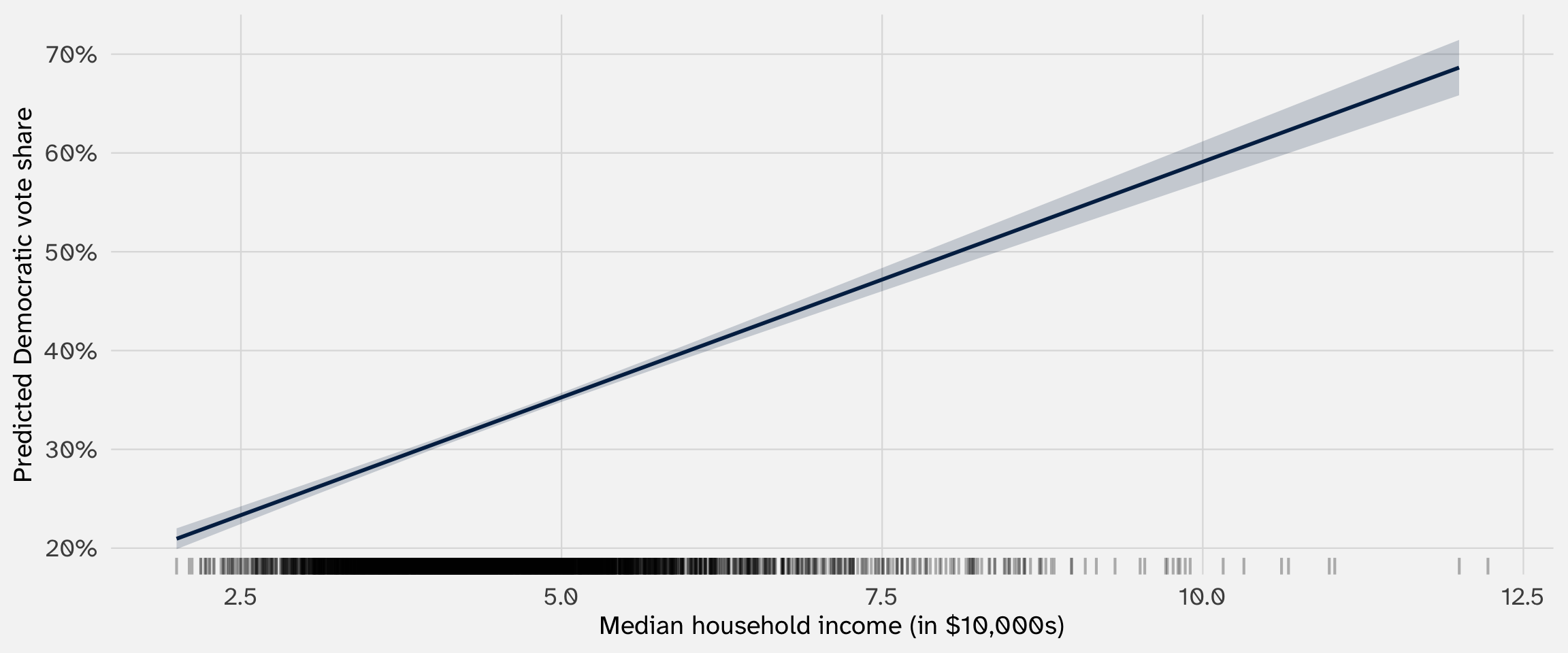
visualize the distribution of X
geom_rug() will show you the distribution of income
The effect of income is always constant
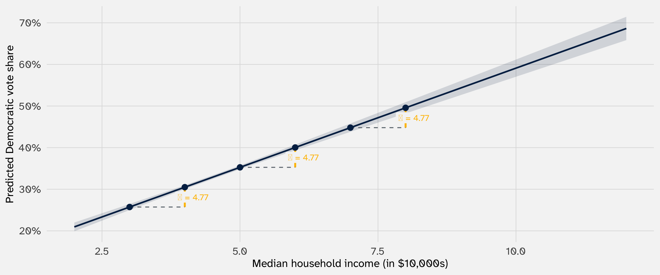
Move anywhere along the line: a $10k increase in income always changes vote share by β = 4.77 percentage points
This is because income is linear (untransformed) in our model
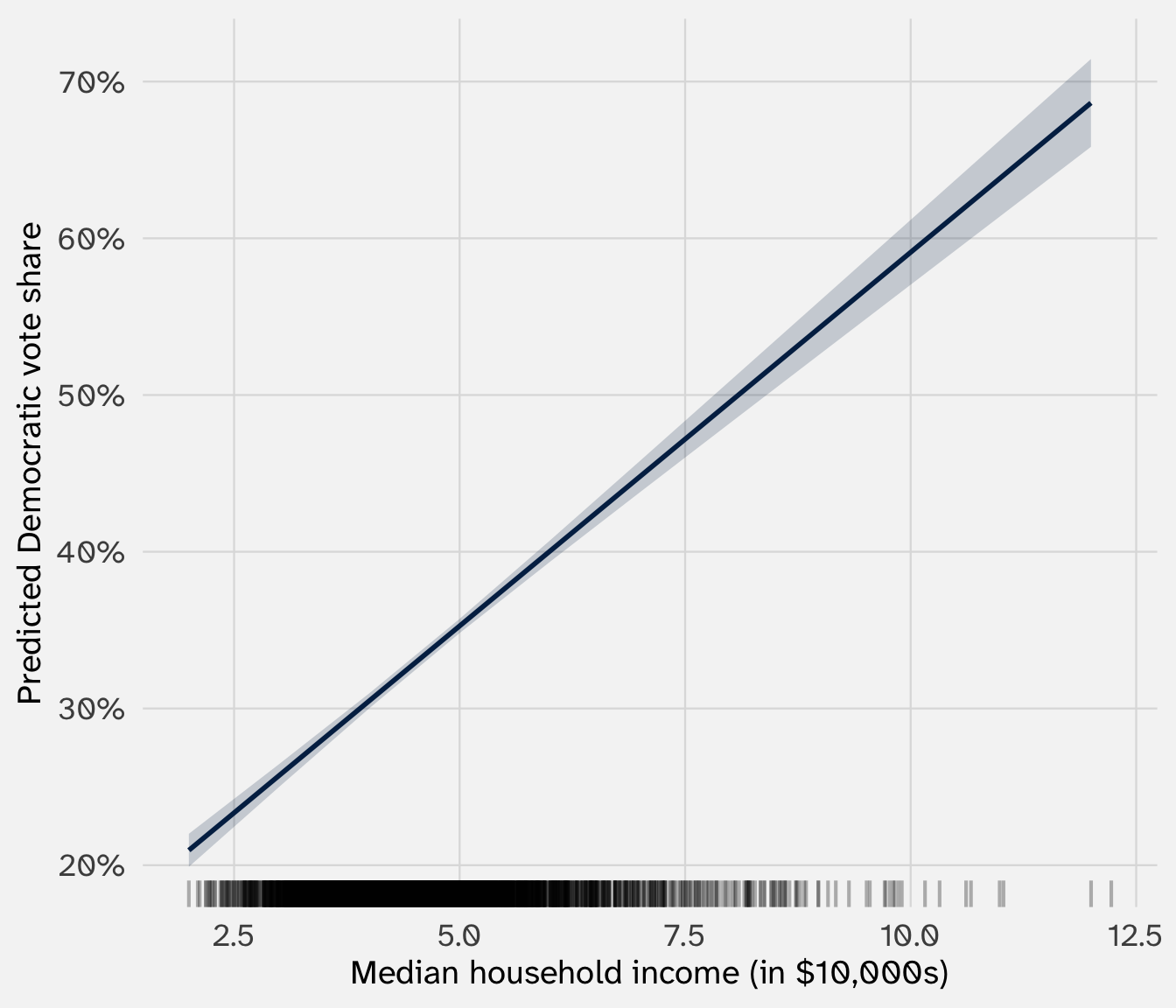
Even with constant effects, visualization earns its keep
If the effect is simply \(\beta\) why visualize?
Even when the effect is constant, visualization shows you:
- Where in the data you have coverage
- The uncertainty across the range of \(X\)
- Whether predictions go out of bounds
For most models, the effect is not just \(\beta\)—visualization will become necessary
Building the calculus + visualization habit now pays off when the models get harder
📝 Activity: constant across controls
We just showed the effect of income is the same no matter where you are in the income distribution—let’s show the same is true for controls
Steps:
- Use
crossing()to build a grid where both income and one control variable vary - Generate predictions with
augment() - Plot the marginal effect of income with separate lines across your chosen control variable
We know what OLS estimates. Now the how—what problem is lm() actually solving?
An optimization problem
Our fitted model
The data:
| name | state | per_dem_2020 | income_10k | white_pct | black_pct |
|---|---|---|---|---|---|
| Autauga County | AL | 27.02 | 5.37 | 78.1 | 18.4 |
| Baldwin County | AL | 22.41 | 5.02 | 87.3 | 9.5 |
| Barbour County | AL | 45.79 | 3.29 | 50.2 | 47.6 |
| Bibb County | AL | 20.70 | 3.64 | 76.3 | 22.1 |
| Blount County | AL | 9.57 | 4.41 | 96.0 | 1.8 |
| Bullock County | AL | 74.70 | 3.20 | 27.2 | 69.9 |
Our model of the data:
\[\text{dem\_pct}_i = \beta_0 + \beta_1 \cdot \text{income\_10k}_i + \beta_2 \cdot \text{white\_pct}_i + \beta_3 \cdot \text{black\_pct}_i + \varepsilon_i\]
We can think of model fitting as an optimization problem: what are the values for \(\beta\) that will fit the data “best”
Intuition: one data point, one answer
Let’s build up the intuition slowly:
Imagine we had only one county, and let’s forget the intercept (\(\beta_0\)) and the control variables:
| name | state | per_dem_2020 | income_10k | white_pct | black_pct |
|---|---|---|---|---|---|
| Autauga County | AL | 27.02 | 5.37 | 78.1 | 18.4 |
\[\text{dem\_pct}_i = \beta_1 \cdot \text{income\_10k}_i + \varepsilon_i\]
What does \(\beta_1\) have to be here?
Two data points: trade-offs
What happens when we add another data point?
| name | state | per_dem_2020 | income_10k | white_pct | black_pct |
|---|---|---|---|---|---|
| Autauga County | AL | 27.02 | 5.37 | 78.1 | 18.4 |
| Baldwin County | AL | 22.41 | 5.02 | 87.3 | 9.5 |
\[\text{dem\_pct}_i = \beta_1 \cdot \text{income\_10k}_i + \varepsilon_i\]
| name | state | per_dem_2020 | income_10k | white_pct | black_pct | residual_beta_5 | residual_beta_4 |
|---|---|---|---|---|---|---|---|
| Autauga County | AL | 27.02 | 5.37 | 78.1 | 18.4 | 0.02 | 3.08 |
| Baldwin County | AL | 22.41 | 5.02 | 87.3 | 9.5 | -2.85 | 0.01 |
With more than one data point, there is no longer a single value that satisfies the equation
And if we are estimating more than one parameter (\(\beta_0, \beta_1, \beta_2, \dots\)) the challenge grows
Our choice of \(\beta\)s must balance these trade-offs—try to fit all data points “as well as possible”
What do we mean by “fit well”?
All models fit parameters to data by optimizing some measure of fit—a criterion for defining what it means for the model to fit the data “well”
This criteria is called a loss function—a metric that describes how wrong a model’s predictions are. Different models use different loss functions
OLS uses one kind of loss function—let’s develop it intuitively
OLS defines “good fit” through residuals
What was our intuition of “good fit” in the two observation example?
| name | state | per_dem_2020 | income_10k | white_pct | black_pct | residual_beta_5 | residual_beta_4 |
|---|---|---|---|---|---|---|---|
| Autauga County | AL | 27.02 | 5.37 | 78.1 | 18.4 | 0.02 | 3.08 |
| Baldwin County | AL | 22.41 | 5.02 | 87.3 | 9.5 | -2.85 | 0.01 |
That the difference between \(Y\) and \(\widehat{Y}\) across our observations should be as small as possible
This difference is known as the residual (\(Y - \widehat{Y}\))
Residual → “residue” → what’s left over
Residuals measure how wrong each prediction is
| income_10k | white_pct | black_pct | per_dem_2020 | .fitted | .resid |
|---|---|---|---|---|---|
| 5.37 | 78.1 | 18.4 | 27.02 | 41.75 | -14.73 |
| 5.02 | 87.3 | 9.5 | 22.41 | 34.36 | -11.95 |
| 3.29 | 50.2 | 47.6 | 45.79 | 49.29 | -3.50 |
| 3.64 | 76.3 | 22.1 | 20.70 | 34.69 | -14.00 |
| 4.41 | 96.0 | 1.8 | 9.57 | 26.05 | -16.48 |
| 3.20 | 27.2 | 69.9 | 74.70 | 63.22 | 11.49 |
Positive residuals → \((Y - \widehat{Y}) \gt 0\) → model under-predicts county Democratic vote share
Negative residuals → \((Y - \widehat{Y}) \lt 0\) → model over-predicts county Democratic vote share
Large residuals are counties the model fits (relatively) poorly
Small residuals are counties the model fits (relatively) well
Intuitively a set of \(\beta\) that produce smaller residuals will fit the data better than a set that produces larger residuals
Look at your residuals
augment() will also give you back residuals for the data used to fit your model:
# A tibble: 3,111 × 11
   .rownames per_dem_2020 income_10k white_pct black_pct .fitted .resid     .hat
   <chr>            <dbl>      <dbl>     <dbl>     <dbl>   <dbl>  <dbl>    <dbl>
 1 1                27.0        5.37      78.1      18.4    41.7 -14.7  0.000696
 2 2                22.4        5.02      87.3       9.5    34.4 -12.0  0.000397
 3 3                45.8        3.29      50.2      47.6    49.3  -3.50 0.00265
 4 4                20.7        3.64      76.3      22.1    34.7 -14.0  0.000726
 5 5                 9.57       4.41      96         1.8    26.1 -16.5  0.000485
 6 6                74.7        3.20      27.2      69.9    63.2  11.5  0.00596
 7 7                41.8        2.99      54.3      43.6    45.3  -3.52 0.00234
 8 8                29.8        4.00      76        20.9    36.5  -6.68 0.000570
 9 9                41.6        3.24      58.8      39.1    43.7  -2.04 0.00183
10 10               13.2        3.49      93.2       4.5    23.4 -10.2  0.000731
# ℹ 3,101 more rows
# ℹ 3 more variables: .sigma <dbl>, .cooksd <dbl>, .std.resid <dbl>Raw residuals can be misleading
Let’s look at our full model again:
\[\text{dem\_pct}_i = \beta_0 + \beta_1 \cdot \text{income\_10k}_i + \beta_2 \cdot \text{white\_pct}_i + \beta_3 \cdot \text{black\_pct}_i + \varepsilon_i\]
Let’s compare three candidate sets of \(\beta\)—which fits best?
| Candidate | β₀ | β₁ | β₂ | β₃ | Sum of residuals |
|---|---|---|---|---|---|
| Set 1 | 60 | 4 | -0.1 | 0.2 | -119302.9 |
| Set 2 | 30 | 3 | -0.3 | 0.5 | 32904.3 |
| Set 3 | 18 | -5 | 0.5 | -0.5 | 0.0 |
Candidate 3 fits best on residuals but looks worst
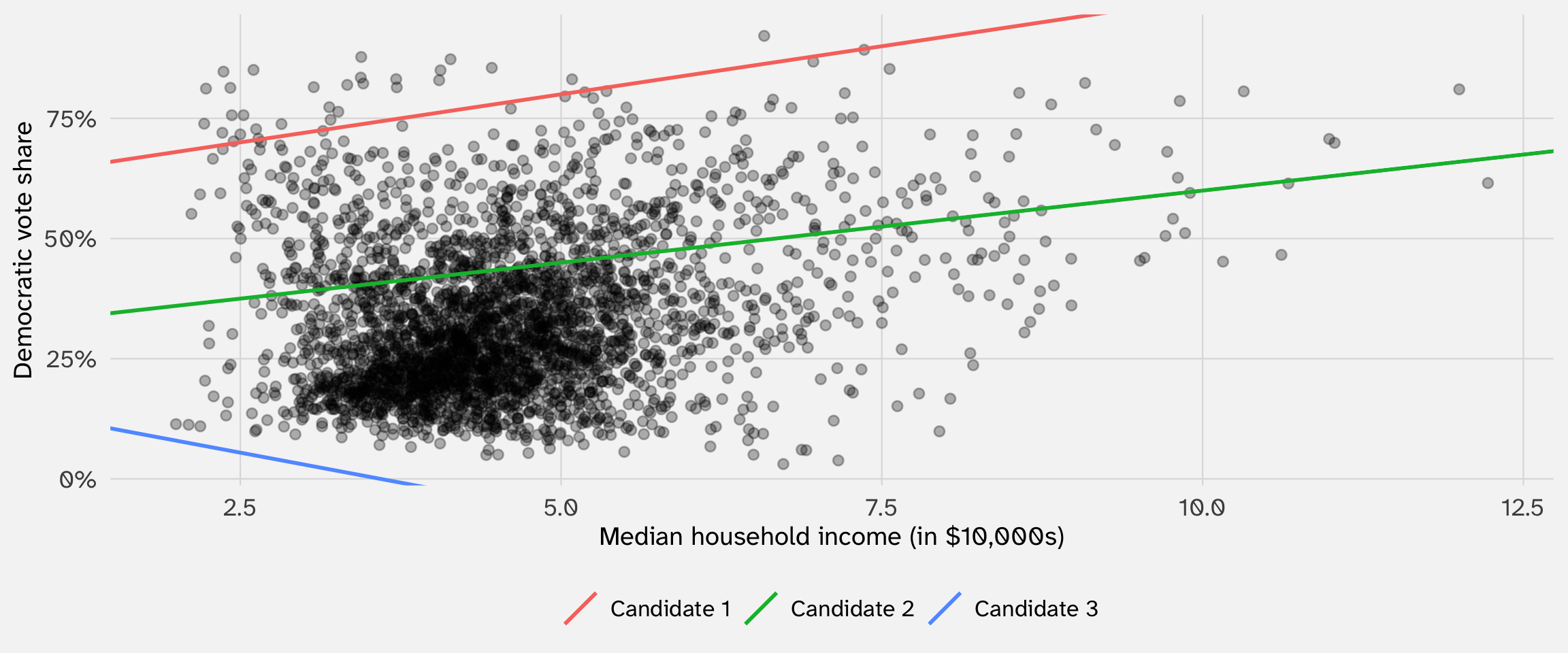
Candidate 3 was our best line—what’s wrong here?
Squaring solves two problems
Problem 1: Positive and negative residuals cancel out
- A line that overshoots some points and undershoots others can have residuals that sum to zero—even if it fits terribly
- Squaring makes every residual positive, so nothing cancels
Problem 2: We want to penalize big misses more than small ones
- A residual of 10 is not just twice as bad as a residual of 5—it’s much worse
- Squaring amplifies large errors: \(10^2 = 100\) vs. \(5^2 = 25\) (4x, not 2x)
This is why OLS minimizes the sum of squared residuals (SSR)
Squared residuals correctly penalize systematic error
Same three candidates, now with squared residuals:
| Candidate | β₀ | β₁ | β₂ | β₃ | Sum of squared residuals |
|---|---|---|---|---|---|
| Set 1 | 60 | 4 | -0.1 | 0.2 | 5133836.4 |
| Set 2 | 30 | 3 | -0.3 | 0.5 | 868820.7 |
| Set 3 | 18 | -5 | 0.5 | -0.5 | 2356416.9 |
Set 3 scored 0.0 on raw residuals but doesn’t win on SSR—squaring prevents positive and negative errors from canceling out
OLS is an optimization problem
So now we know what we need to optimize over—we need to find the set of \(\beta\) that will minimize the sum of squared residuals:
\[\sum_{i=1}^n (Y_i - \widehat{Y}_i)^2\]
Remember that \(\widehat{Y}_i = \widehat{\beta}_0 + \widehat{\beta}_1 X_i\)
So can rewrite: \(\sum_{i=1}^n (Y_i - \widehat{Y}_i)^2 = \sum_{i=1}^n (Y_i - \widehat{\beta}_0 - \widehat{\beta}_1 X_i)^2\)
So we need to pick \(\beta_0\) and \(\beta_1\) to make this as small as possible (minimize):
\[\sum_{i=1}^n (Y_i - \widehat{\beta}_0 - \widehat{\beta}_1 X_i)^2\]
Some models have formulas; some need search
There are two broad classes of modeling approaches:
Statistical theory make assumptions and use math to find the set of \(\beta\) that minimize the loss function - these typically have a closed-form solution—there is one set of \(\beta\) that minimize the loss function - that set can be mathematically derived
Computational / numerical approaches use constrained, educated guessing to identify the set of \(\beta\) - these typically do not have a closed-form solution—there is no way to nicely derive the set of \(\beta\) that minimize the loss function
OLS has a closed-form solution
We can use calculus (or matrix algebra) to find the values for \(\beta\) that will minimize the sum of squared residuals
Three steps: write the loss, differentiate, solve
The recipe for finding a minimum is the same one from calculus:
- Write down the thing you want to minimize (the loss function)
- Take the derivative with respect to the thing you’re choosing (\(\beta\))
- Set it equal to zero and solve
If you can do these three steps, you can derive OLS.
Step 1: Write down the loss function
One predictor, with intercept. The model is \(\widehat{Y}_i = \beta_0 + \beta_1 X_i\)
The sum of squared residuals is:
\[SSR(\beta_0, \beta_1) = \sum_{i=1}^{n}(Y_i - \beta_0 - \beta_1 X_i)^2\]
This is a function of two unknowns: \(\beta_0\) and \(\beta_1\). Everything else (\(Y_i\), \(X_i\)) is data we observe
We’ll focus on \(\beta_1\)
Step 2: Take the partial derivative
We want \(\hat{\beta}_1\), so differentiate w.r.t. \(\beta_1\), treating \(\beta_0\) as a constant:
\[\frac{\partial \, SSR}{\partial \beta_1} = \sum_{i=1}^{n}(Y_i - \beta_0 - \beta_1 X_i)^2\]
The chain rule says: take the derivative of the outer, then multiply by the derivative of the inner
Derivative of the outer: \[(Y_i - \beta_0 - \beta_1 X_i)^2 \rightarrow 2(Y_i - \beta_0 - \beta_1 X_i)\]
Derivative of the inner: \[(Y_i - \beta_0 - \beta_1 X_i) \rightarrow -X_i\]
Multiply outer \(\times\) inner and simplify: \[= -2\sum_{i=1}^n X_i(Y_i - \beta_0 - \beta_1 X_i)\]
Step 3: Set equal to zero and solve
\[-2\sum_{i=1}^n X_i(Y_i - \beta_0 - \beta_1 X_i) = 0\]
Divide by \(-2\) and distribute:
\[\sum_{i=1}^n X_i Y_i - \beta_0 \sum_{i=1}^n X_i - \beta_1 \sum_{i=1}^n X_i^2 = 0\]
We have one equation but two unknowns (\(\beta_0\) and \(\beta_1\))—we need to know what \(\beta_0\) equals before we can solve for \(\beta_1\)
On the problem set, you will show that:
\[\hat{\beta}_0 = \bar{Y} - \hat{\beta}_1 \bar{X}\]
Quick detour: two equations, two unknowns
Suppose you have two equations and two unknowns (\(a\) and \(b\)):
\[ \begin{align} 2a + b &= 10 \quad \text{...(1)}\\ a - b &= 2 \quad \text{...(2)} \end{align} \]
Step 1 — Solve one equation for one unknown. From (2): \(\; b = a - 2\)
Step 2 — Substitute into the other. Plug into (1): \(\; 2a + (a-2) = 10 \implies 3a = 12 \implies a = 4\)
Step 3 — Back-substitute. \(\; b = 4 - 2 = 2\)
The answer for \(a\) temporarily depended on \(b\)—but substitution removed that dependence. We’ll use the exact same trick now.
Step 3 (continued): Substitute and solve
We had: \(\sum X_i Y_i - \beta_0 \sum X_i - \beta_1 \sum X_i^2 = 0\)
Substitute \(\hat{\beta}_0 = \bar{Y} - \hat{\beta}_1 \bar{X}\):
\[\sum X_i Y_i - (\bar{Y} - \hat{\beta}_1 \bar{X}) \sum X_i - \hat{\beta}_1 \sum X_i^2 = 0\]
Distribute \(\sum X_i\) into the parenthetical:
\[\sum X_i Y_i - \bar{Y}\sum X_i + \hat{\beta}_1 \bar{X}\sum X_i - \hat{\beta}_1 \sum X_i^2 = 0\]
Replace \(\sum X_i\) with \(n\bar{X}\):
\[\sum X_i Y_i - n\bar{X}\bar{Y} + \hat{\beta}_1 n\bar{X}^2 - \hat{\beta}_1 \sum X_i^2 = 0\]
Step 3 (end): The OLS estimator
Move the \(\hat{\beta}_1\) terms to the right:
\[\sum X_i Y_i - n\bar{X}\bar{Y} = \hat{\beta}_1 \sum X_i^2 - \hat{\beta}_1 n\bar{X}^2\]
Factor out \(\hat{\beta}_1\):
\[\sum X_i Y_i - n\bar{X}\bar{Y} = \hat{\beta}_1 \left(\sum X_i^2 - n\bar{X}^2\right)\]
The left side can be rewritten as \(\sum(X_i - \bar{X})(Y_i - \bar{Y})\) = \(Cov(X, Y)\);
the right side can be rewritten as \(\sum(X_i - \bar{X})^2\) = \(Var(X)\)
\[\boxed{\hat{\beta}_1 = \frac{\sum_{i=1}^n (X_i - \bar{X})(Y_i - \bar{Y})}{\sum_{i=1}^n (X_i - \bar{X})^2}}\]
This is the OLS slope estimate. Plug in data, get an answer. No guessing, no iteration.
The formula and lm() give the same answer
We can compute \(\hat{\beta}_1\) directly from the data using the formula we just derived:
[1] 3.317128Same thing using lm():
The formula on the board and the number R gives you are the same thing—no black box.
Multiple predictors: same recipe, matrix bookkeeping
We derived \(\hat{\beta}_1\) for one predictor. With multiple predictors (\(\beta_0, \beta_1, \ldots, \beta_k\)), the recipe is the same—take partial derivatives, set to zero—but the system of equations grows
We use matrix algebra to write and solve that system compactly:
\[SSR(\boldsymbol{\beta}) = \sum_{i=1}^n(Y_i - \mathbf{x}_i'\boldsymbol{\beta})^2\]
Differentiate, set to zero, solve \(\rightarrow\) the normal equations:
\[\hat{\boldsymbol{\beta}} = (\mathbf{X}'\mathbf{X})^{-1}\mathbf{X}'\mathbf{y}\]
You don’t need to memorize this. The recipe is the same—the matrices are just bookkeeping for handling \(k\) unknowns at once. The point is that a closed-form solution exists.
The big picture
- A model is a recipe for predicting \(Y\) from \(X\)—the coefficients (\(\beta\)) are the ingredients
- OLS finds the \(\beta\) that minimize the sum of squared residuals—a closed-form solution exists
- For linear models, the effect of \(X\) equals its coefficient—but this convenience disappears with transformations and non-linear models
- We interpret effects using calculus (what’s the formula?) and visualization (what does it mean in context?)
- This course: models where there is no closed-form solution—we’ll need to search for the optimum numerically (maximum likelihood)
Appendix: extra slides
(Cover only if time permits)
Why does the recipe work?
Hold \(\beta_0\) fixed and think of SSR as a function of \(\beta_1\) alone. Expand the square:
\[SSR(\beta_1) = \sum_{i=1}^n (Y_i - \beta_0 - \beta_1 X_i)^2\]
Collecting terms by powers of \(\beta_1\), this has the form:
\[SSR(\beta_1) = \underbrace{\sum X_i^2}_{a}\;\beta_1^2 \;-\; \underbrace{2\sum X_i (Y_i - \beta_0)}_{b}\;\beta_1 \;+\; \underbrace{\text{constants}}_{c}\]
This is \(a\beta_1^2 - b\beta_1 + c\)—a parabola that opens upward (because \(a > 0\))
Parabolas have exactly one minimum, which is why the derivative-equals-zero trick gives us a unique answer
What does “quadratic in \(\beta_1\)” look like?
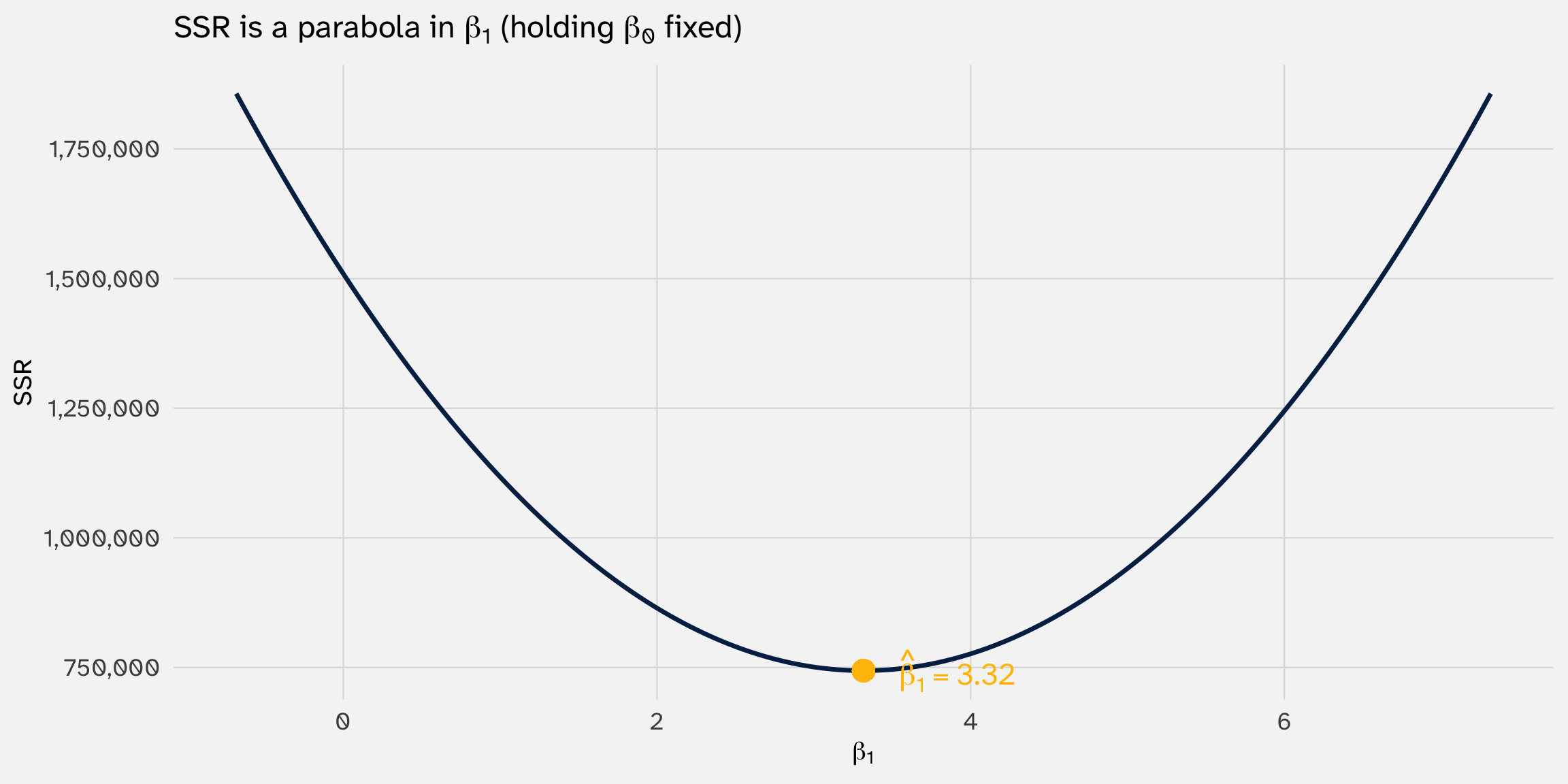
Every value of \(\beta_1\) maps to a single SSR. The curve is smooth, U-shaped, and has one bottom. That’s why calculus works here.
Activity: why not absolute residuals?
If the problem with summing residuals was that negatives cancel positives—why not just take the absolute value?
\[\text{SAR}(\beta) = \sum_{i=1}^n |Y_i - \beta X_i|\]
Here are 5 counties from our data:
| County | State | X (income, x$10k) | Y (Dem %) |
|---|---|---|---|
| Buchanan County | MO | 4.4 | 36.7 |
| Shelby County | TN | 4.6 | 64.4 |
| San Juan County | CO | 4.0 | 60.7 |
| St. Louis County | MN | 4.7 | 56.6 |
| Roane County | WV | 2.9 | 25.2 |
Compute \(\text{SAR}(\beta)\) for \(\beta = 5\), \(\beta = 7\), and \(\beta = 9\). Which \(\beta\) gives the smallest SAR?
SAR has kinks; SSR is smooth
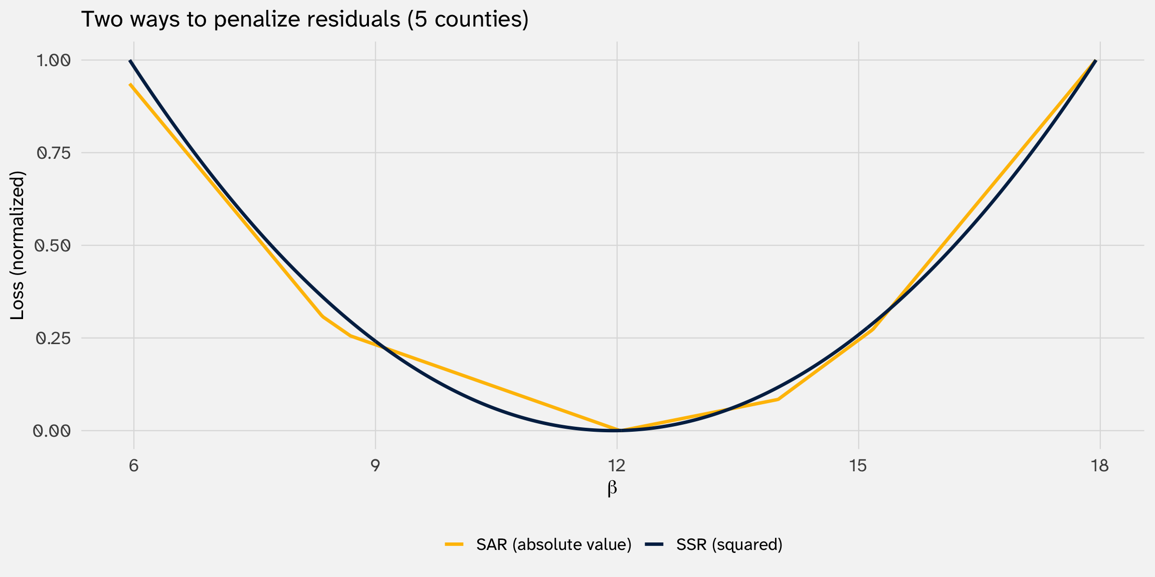
SSR is a smooth parabola; SAR has kinks (piecewise linear)
Kinks = not differentiable → can’t just “set the derivative to zero”
Why squaring wins
Squaring residuals isn’t arbitrary—it gives us a smooth, convex objective function
Smooth → we can take derivatives and set them to zero
Convex (parabola) → exactly one minimum, no ambiguity
These properties are what make the OLS formula \((\mathbf{X}'\mathbf{X})^{-1}\mathbf{X}'\mathbf{y}\) work
Most models in this course (logit, Poisson, duration) will also have smooth, concave objective functions—but no closed-form solution
We’ll have to search for the optimum numerically—that’s what maximum likelihood estimation is all about