| name | state | hh_income | income_10k |
|---|---|---|---|
| Autauga County | AL | 53682 | 5.37 |
| Baldwin County | AL | 50221 | 5.02 |
| Barbour County | AL | 32911 | 3.29 |
| Bibb County | AL | 36447 | 3.64 |
| Blount County | AL | 44145 | 4.41 |
| Bullock County | AL | 32033 | 3.20 |
Common Transformations
POL 213 · Week 2
Juan F. Tellez
University of California, Davis
April 8, 2026
Housekeeping
- PS1
- Extra problems for methods
- Group project pairs
Where we are
Last week: OLS as an optimization problem (minimize SSR), effects via calculus and visualization
The effect of \(X\) on \(Y\) was simply the coefficient \(\beta\)—constant across all values of \(X\)
This week: what happens when we transform the variables in our model?
Key idea: transformations can change the shape of the effect → the coefficient alone is less useful
Linear transformations
Change the units; story stays the same
- rescaling Y, X
- standardization
Scale transformations don’t change the shape (constant)
scale transformations change the scale: the coefficient changes size, but the effect is still linear and constant
We did this week 1 with household income:
Same model, different ruler
These are useful for interpretability
How did dividing income by 10,000 change \(\beta\)?
| term | estimate | std.error | statistic | p.value |
|---|---|---|---|---|
| (Intercept) | 0.180672 | 0.011116 | 16.25398 | 0 |
| hh_income | 0.000003 | 0.000000 | 14.11011 | 0 |
| term | estimate | std.error | statistic | p.value |
|---|---|---|---|---|
| (Intercept) | 0.180672 | 0.011116 | 16.25398 | 0 |
| income_10k | 0.033171 | 0.002351 | 14.11011 | 0 |
The coefficient grew by a factor of 10,000 — but notice the \(t\)-statistic and \(p\)-value are identical
Other model statistics (such as \(R^2\)) remain identical
| Model | R² |
|---|---|
| Raw dollars | 0.060184 |
| $10,000s | 0.060184 |
Same logic for the outcome
What if we rescale \(Y\) instead? Express Democratic vote share as a percent (0–100) instead of a proportion (0–1):
Y as proportion
| term | estimate | std.error | statistic | p.value |
|---|---|---|---|---|
| (Intercept) | 0.1806723 | 0.0111156 | 16.25398 | 0 |
| hh_income | 0.0000033 | 0.0000002 | 14.11011 | 0 |
Y as percent
| term | estimate | std.error | statistic | p.value |
|---|---|---|---|---|
| (Intercept) | 18.0672310 | 1.1115572 | 16.25398 | 0 |
| hh_income | 0.0003317 | 0.0000235 | 14.11011 | 0 |
Coefficient grows by a factor of 100 — \(t\)-statistic and \(p\)-value still identical
Rescaling: why it’s “free”
Say we measure income in thousands instead of dollars: \(\tilde{X} = X / 1000\)
Remember OLS is just: \(\hat{\beta} = \frac{\text{Cov}(X,\, Y)}{\text{Var}(X)}\)
What happens when we plug in \(\tilde{X}\)?
- Numerator: \(\text{Cov}(X/1000,\, Y) = \frac{1}{1000}\text{Cov}(X,Y)\) — shrinks by 1,000
- Denominator: \(\text{Var}(X/1000) = \frac{1}{1000^2}\text{Var}(X)\) — shrinks by 1,000,000
Dividing: \(\hat{\tilde{\beta}} = \frac{\text{shrinks by } 1000}{\text{shrinks by } 1000^2} = 1000 \times \hat{\beta}\)
The coefficient gets bigger by exactly the factor we divided \(X\) by — the predictions stay the same, and so do \(t\)-statistics and \(p\)-values (the SE scales by the same factor)
Standardization: comparing apples to apples
Suppose an experiment randomly assigns a political prime (vs. control). Three outcomes:
| Outcome | Scale | Units |
|---|---|---|
| Feeling thermometer | 0–100 | degrees |
| Support for policy | 1–7 | Likert scale |
| Petition signatures | 0–∞ | count |
Where did the treatment have the biggest effect?
Simulating the experiment
| treated | thermometer | support | petitions |
|---|---|---|---|
| 0 | 41.42 | 2.22 | 2 |
| 0 | 17.77 | 3.67 | 3 |
| 1 | 74.76 | 4.62 | 5 |
| 0 | 83.05 | 4.67 | 2 |
| 1 | 18.03 | 5.83 | 8 |
modelsummary(
  list("Thermometer" = lm(thermometer ~ treated, data = experiment),
       "Policy support" = lm(support ~ treated, data = experiment),
       "Petitions" = lm(petitions ~ treated, data = experiment)), stars = TRUE, gof_omit = "IC|Log|Adj|F|RMSE|Num", coef_rename = c("(Intercept)" = "Intercept", "treated" = "Treatment")
)| Thermometer | Policy support | Petitions | |
|---|---|---|---|
| + p < 0.1, * p < 0.05, ** p < 0.01, *** p < 0.001 | |||
| Intercept | 49.134*** | 3.905*** | 2.840*** |
| (2.142) | (0.114) | (0.201) | |
| Treatment | 8.775** | 0.812*** | 2.000*** |
| (3.029) | (0.161) | (0.284) | |
| R2 | 0.041 | 0.114 | 0.201 |
Raw coefficients are misleading
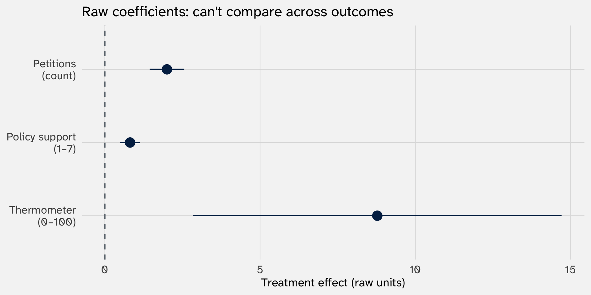
The thermometer “wins” — but only because it has the widest scale. This comparison is meaningless
The fix: standardize each outcome
Standardizing = subtract the mean, divide by the SD: \(Z_i = \frac{Y_i - \bar{Y}}{s_Y}\)
Step 1: subtract the mean. Now every outcome is centered at zero → a score of 5 means “5 above average.” But “5 above average” on a 100-point thermometer is tiny, while “5 above average” on a 7-point scale is huge. The scales are still different
Step 2: divide by the SD. The standard deviation measures how much a variable typically varies. Dividing by it answers: “how many typical spreads is this value from the mean?” A thermometer score 1 SD above the mean is as unusual as a petition count 1 SD above its mean → regardless of whether that’s 20 degrees or 3 signatures
After both steps, every variable is in the same units: “number of standard deviations from the mean.” The original scale — degrees, Likert points, counts is gone
Now we can compare
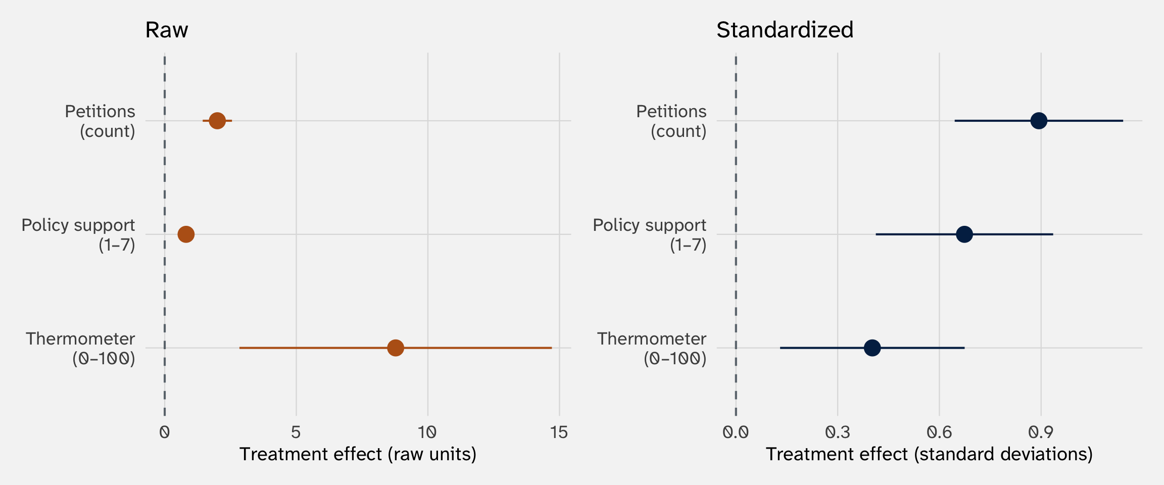
On a common scale, the treatment moved petitions the most (in SD units) — the raw numbers hid this because petition counts have a tight distribution
Standardizing lets you ask: “where did the treatment move the needle most, relative to how much the outcome varies?”
Testing for an overall effect
Once outcomes share a common scale, we can go further: average them into a single index
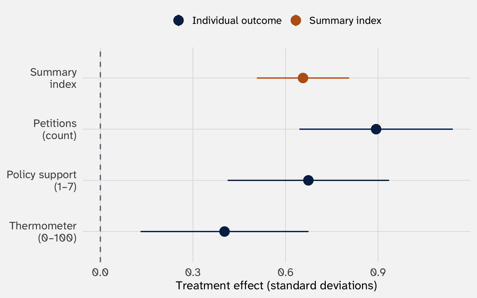
The summary index gives us a single test of whether the treatment increased political engagement overall → addresses multiple-testing concerns
Nonlinear transformations
Change the shape of the relationship between X and Y
Nonlinear effects: A working example
Question Does democratization fuel or suppress protest?
Premise 1 In full autocracies, repression prevents collective action
Premise 2 In full democracies, institutional channels reduce the need for street protest
Expectation Protest should increase as countries move away from autocracy—up to a point—before decreasing
This is an old idea in comparative politics: the “more violence in the middle” pattern (Muller and Weede 1990)
It is also a theory of a nonlinear effect → the effect of democratization on protest varies
The data: V-Dem
| country | year | democracy | mobilization | ln_gdppc | ln_pop |
|---|---|---|---|---|---|
| Mexico | 1946 | 0.19 | -0.94 | 1.89 | 7.84 |
| Sweden | 1946 | 0.76 | -1.75 | 2.97 | 6.54 |
| Ghana | 1946 | 0.10 | 0.57 | 1.47 | 6.21 |
| South Africa | 1946 | 0.23 | 1.69 | 2.32 | 6.81 |
| Japan | 1946 | 0.31 | -1.46 | 1.81 | 8.99 |
| Burma/Myanmar | 1946 | 0.17 | 0.39 | 0.52 | 7.53 |
Outcome mobilization — frequency and size of mass mobilization events (continuous latent scale)
Treatment democracy — V-Dem electoral democracy index (0–1)
Controls ln(GDP per capita), ln(population)
A quadratic term allows the effect of democracy to vary
Add \(\text{democracy}^2\) to the model:
\[\text{mobilization}_i = \beta_0 + \beta_1 \cdot \text{dem}_i + \beta_2 \cdot \text{dem}_i^2 + \beta_3 \cdot \ln(\text{gdppc})_i + \beta_4 \cdot \ln(\text{pop})_i + \varepsilon_i\]
What is the effect of democracy on protest?
| Quadratic | |
|---|---|
| + p < 0.1, * p < 0.05, ** p < 0.01, *** p < 0.001 | |
| Intercept | -2.754*** |
| (0.055) | |
| Democracy | 7.676*** |
| (0.177) | |
| Democracy² | -8.032*** |
| (0.195) | |
| ln(GDP per capita) | -0.044*** |
| (0.013) | |
| ln(Population) | 0.179*** |
| (0.006) | |
| Num.Obs. | 11400 |
| R2 | 0.213 |
We have two democracy terms
The effect now depends on where you are
Last week, the derivative gave us a number. Now it gives us a formula
\[\frac{\partial \hat{Y}}{\partial \text{democracy}} \left[\hat{\beta}_0 + \hat{\beta}_1 \cdot \text{dem} + \hat{\beta}_2 \cdot \text{dem}^2 + \hat{\beta}_3 \cdot \ln(\text{gdppc}) + \hat{\beta}_4 \cdot \ln(\text{pop}) \right]\]
Apply the power and constant rule to each term:
\[= \underbrace{0}_{\text{constant}} + \underbrace{\hat{\beta}_1 \cdot 1}_{\text{power rule}} + \underbrace{2\hat{\beta}_2 \cdot \text{dem}}_{\text{power rule}} + \underbrace{0}_{\text{gdppc fixed}} + \underbrace{0}_{\text{pop fixed}}\]
\[\boxed{\frac{\partial \hat{Y}}{\partial \text{democracy}} = \hat{\beta}_1 + 2\hat{\beta}_2 \cdot \text{democracy}}\]
The effect of democracy on mobilization depends on the current level of democracy
The effect can even change sign
\[\frac{\partial \hat{Y}}{\partial \text{democracy}} = 7.68 + 2(-8.03) \cdot \text{democracy}\]
| Democracy level | Marginal effect | Interpretation |
|---|---|---|
| Autocracy (0.15) | 5.27 | More democracy → more mobilization |
| Hybrid (0.48) | -0.03 | Near the peak → effect ≈ 0 |
| Democracy (0.80) | -5.17 | More democracy → less mobilization |
This is the core lesson: transforming \(X\) means the effect of \(X\) is no longer just \(\beta\)
Compare protest across levels of democracy
Same workflow as week 1: define a scenario, generate predictions, plot
Step 1: Use crossing() to build a grid — vary democracy, hold controls at their means
Predicted mobilization across democracy levels
Step 3: Plot
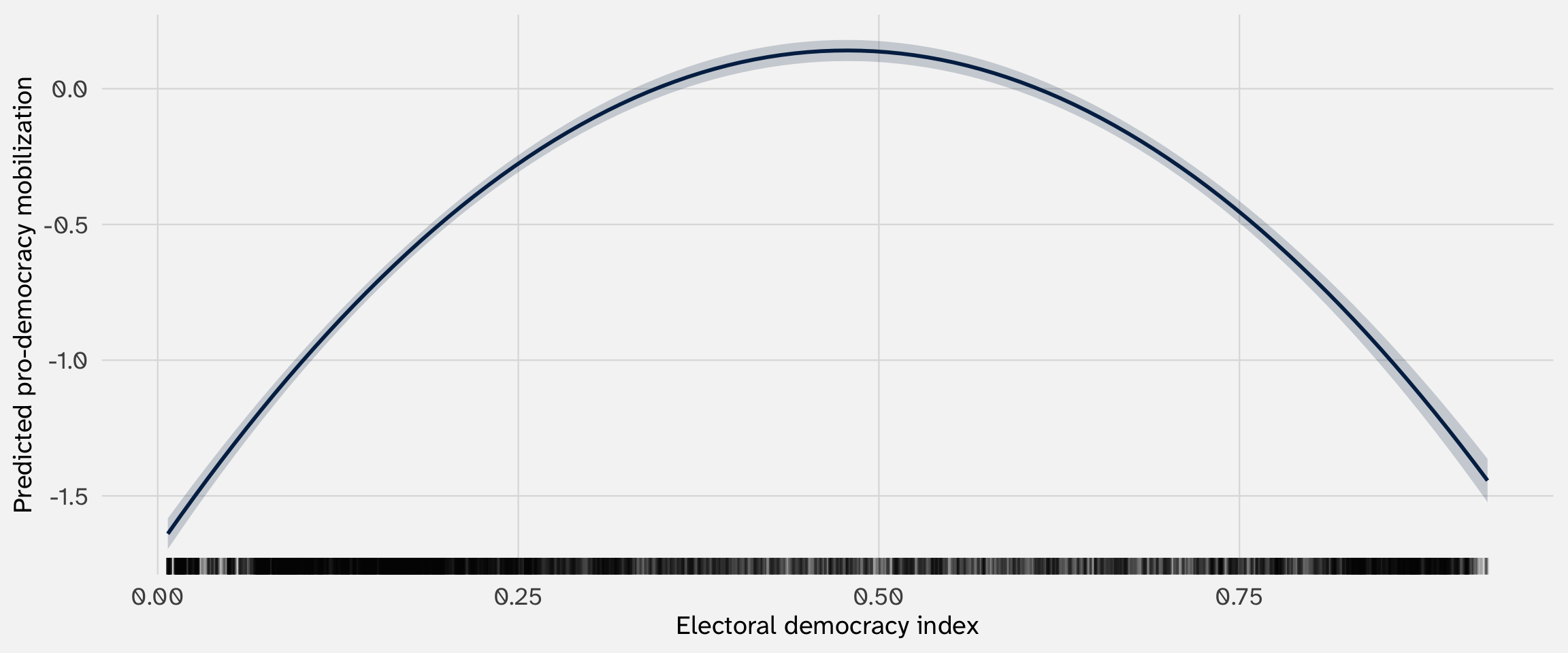
This is a plot of predicted \(\hat{Y}\) — it shows the level of mobilization we expect at each value of democracy
The effect is no longer constant
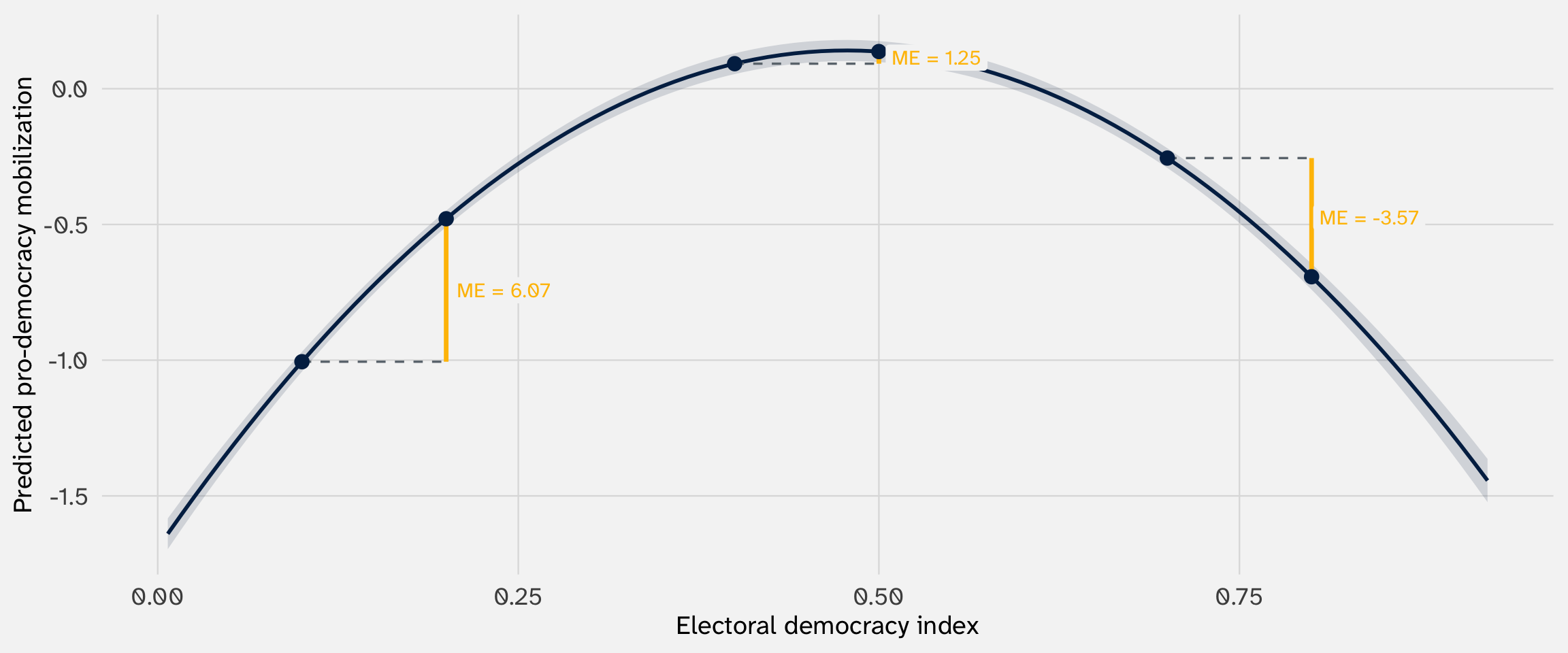
The same \(\Delta X\) produces different \(\Delta Y\) depending on where you start—the effect is a function, not a number
The marginal effect of democracy
We can also visualize how the effect changes as a function of democracy → plug in democracy values into first derivative formula:
\[\frac{\partial \hat{Y}}{\partial \text{democracy}} = 7.68 + 2(-8.03) \cdot \text{democracy}\]
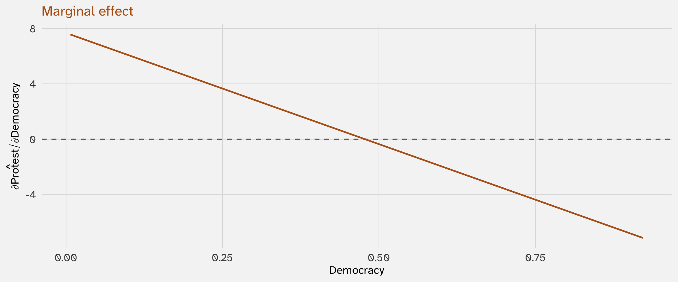
Two different questions, two different plots
Predicted values (augment)
“What level of \(Y\) do we expect at this value of \(X\)?”
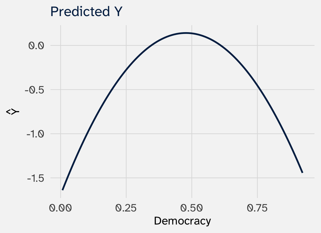
- Shows the shape of the relationship
- Y-axis is in units of the outcome
- Made with
augment()
Marginal effects (slopes)
“How much does \(Y\) change if we increase \(X\) by one unit?”
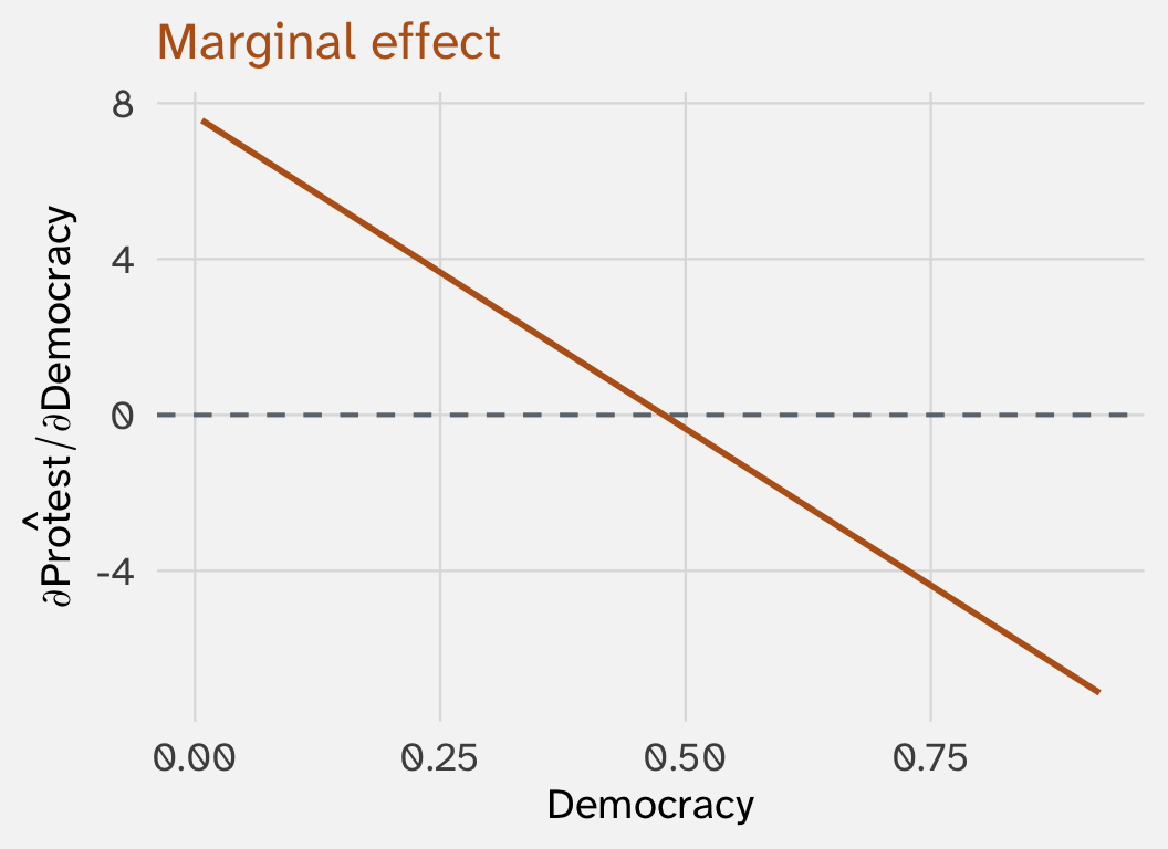
- Shows the slope of the predicted curve at each point
- Y-axis is the derivative: the rate of change
- Made with
slopes()
Where is the peak?
At the peak, the effect is exactly zero—mobilization is neither increasing nor decreasing
Set the marginal effect to zero and solve:
\[\hat{\beta}_1 + 2\hat{\beta}_2 \cdot \text{dem}^* = 0\]
\[\text{dem}^* = \frac{-\hat{\beta}_1}{2\hat{\beta}_2} = \frac{-7.68}{2 \times -8.03} = 0.48\]
The peak occurs at democracy \(\approx 0.48\)—roughly the midpoint of the 0–1 scale
This is consistent with the “more violence in the middle” thesis
Without the quadratic term, the effect is constant
| Linear | Quadratic | |
|---|---|---|
| + p < 0.1, * p < 0.05, ** p < 0.01, *** p < 0.001 | ||
| Intercept | -1.590*** | -2.754*** |
| (0.050) | (0.055) | |
| Democracy | 0.679*** | 7.676*** |
| (0.051) | (0.177) | |
| ln(GDP per capita) | -0.216*** | -0.044*** |
| (0.013) | (0.013) | |
| ln(Population) | 0.196*** | 0.179*** |
| (0.007) | (0.006) | |
| Democracy² | -8.032*** | |
| (0.195) | ||
| Num.Obs. | 11400 | 11400 |
| R2 | 0.096 | 0.213 |
Using calculus (same as last week): \(\frac{\partial \hat{Y}}{\partial \text{democracy}} = \beta_1\) — the effect is constant
Compare: linear vs. quadratic predictions
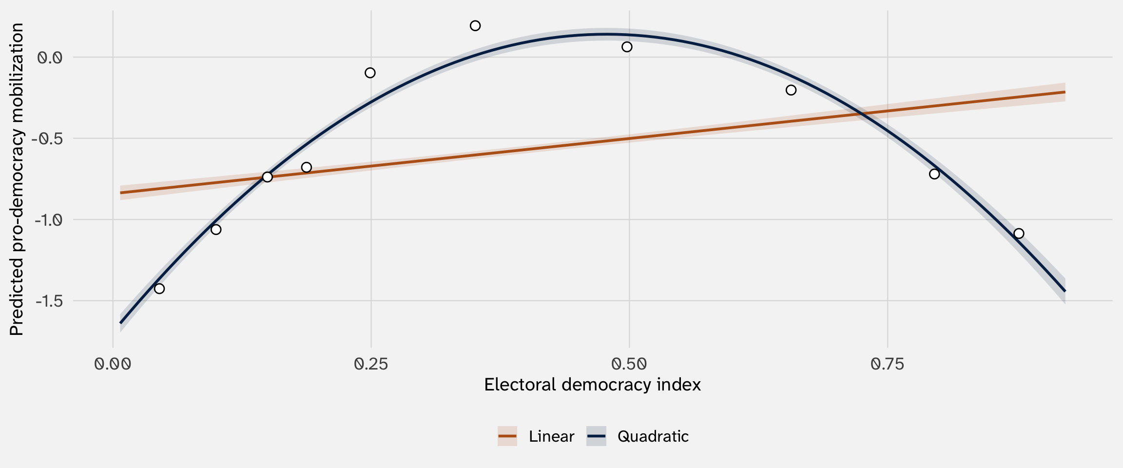
Hollow points are binned means from the raw data. The quadratic captures the shape; the linear model cannot
It’s the specification, not the estimator
Both models are fit with lm() — both are OLS
The difference is the specification: adding \(X^2\) lets the relationship curve
Last week we said:
“It’s the specification that determines whether the effect is constant, not the estimator”
Now we’ve seen this in action. And later in the course, when we use MLE-based models (logit, Poisson), the effects will always depend on covariates—there will be no “constant effect” shortcut
Interactions
The effect of \(X\) depends on \(Z\)
From polynomials to interactions
A polynomial like \(\beta_1 X + \beta_2 X^2\) is really \(X\) interacted with itself—the marginal effect of \(X\) depends on where you are on \(X\)
But often we want to ask: does the effect of \(X\) depend on a different variable \(Z\)?
\(Z\) is called a moderator: it moderates (changes) the relationship between \(X\) and \(Y\)
\[Y_i = \beta_0 + \beta_1 X_i + \beta_2 Z_i + \beta_3 (X_i \times Z_i) + \varepsilon_i\]
The marginal effect of \(X\):
\[\frac{\partial Y}{\partial X} = \beta_1 + \beta_3 \cdot Z_i\]
The effect of \(X\) is no longer a single number—it’s a function of \(Z\)
Example: income and voting in the US
Question: does the effect of county income on the Democratic vote share depend on whether the county is in the South?
\[\text{Dem vote}_i = \beta_0 + \beta_1 \cdot \text{income}_i + \beta_2 \cdot \text{South}_i + \beta_3 \cdot (\text{income}_i \times \text{South}_i) + \varepsilon_i\]
Interpreting the interaction
| No interaction | With interaction | |
|---|---|---|
| + p < 0.1, * p < 0.05, ** p < 0.01, *** p < 0.001 | ||
| Intercept | 0.181*** | 0.082*** |
| (0.012) | (0.017) | |
| Income ($10k) | 0.033*** | 0.054*** |
| (0.002) | (0.004) | |
| South | -0.001 | 0.176*** |
| (0.006) | (0.023) | |
| Income × South | -0.039*** | |
| (0.005) | ||
| Num.Obs. | 3111 | 3111 |
| R2 | 0.060 | 0.079 |
To interpret the effect of income, we’ll need to incorporate the South
Calculus with a binary moderator
\[\frac{\partial \text{Dem vote}}{\partial \text{income}}[\text{Dem vote}_i = \beta_0 + \beta_1 \cdot \text{income}_i + \beta_2 \cdot \text{South}_i + \beta_3 \cdot (\text{income}_i \times \text{South}_i)]\]
\[\frac{\partial \text{Dem vote}}{\partial \text{income}} = \beta_1 + \beta_3 \cdot \text{South}\]
Non-South (South = 0):
\[0.054 + -0.039 \times 0 = 0.054\]
Each additional $10k in income → 0.054 points more Democratic
South (South = 1):
\[0.054 + -0.039 \times 1 = 0.015\]
Each additional $10k in income → 0.015 points more Democratic
Income has a much weaker effect on Democratic voting in the South
Visualizing the interaction
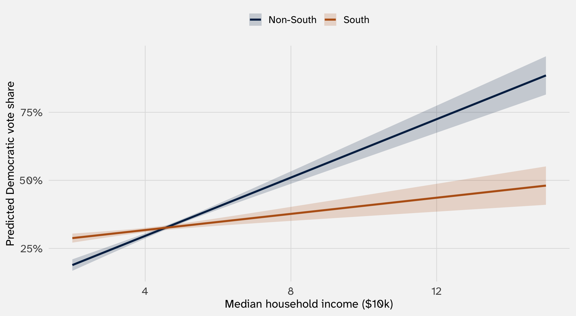
The slopes are different—that’s the interaction
Continuous × continuous: democracy and GDP
With a binary moderator, you get two slopes. With a continuous moderator, the effect changes smoothly
Back to our working example: does the effect of democracy on mobilization depend on how rich the country is?
\[\text{mobilization}_i = \beta_0 + \beta_1 \cdot \text{democracy}_i + \beta_2 \cdot \ln(\text{gdppc})_i + \beta_3 \cdot (\text{democracy}_i \times \ln\text{gdppc}_i) + \beta_4 \cdot \ln(\text{pop})_i + \varepsilon_i\]
Decreasing in GDP
| No interaction | With interaction | |
|---|---|---|
| + p < 0.1, * p < 0.05, ** p < 0.01, *** p < 0.001 | ||
| Intercept | -1.590*** | -2.267*** |
| (0.050) | (0.061) | |
| Democracy | 0.679*** | 2.894*** |
| (0.051) | (0.129) | |
| ln(GDP per capita) | -0.216*** | 0.037* |
| (0.013) | (0.018) | |
| ln(Population) | 0.196*** | 0.199*** |
| (0.007) | (0.007) | |
| Democracy × ln(GDP pc) | -0.720*** | |
| (0.039) | ||
| Num.Obs. | 11400 | 11400 |
| R2 | 0.096 | 0.123 |
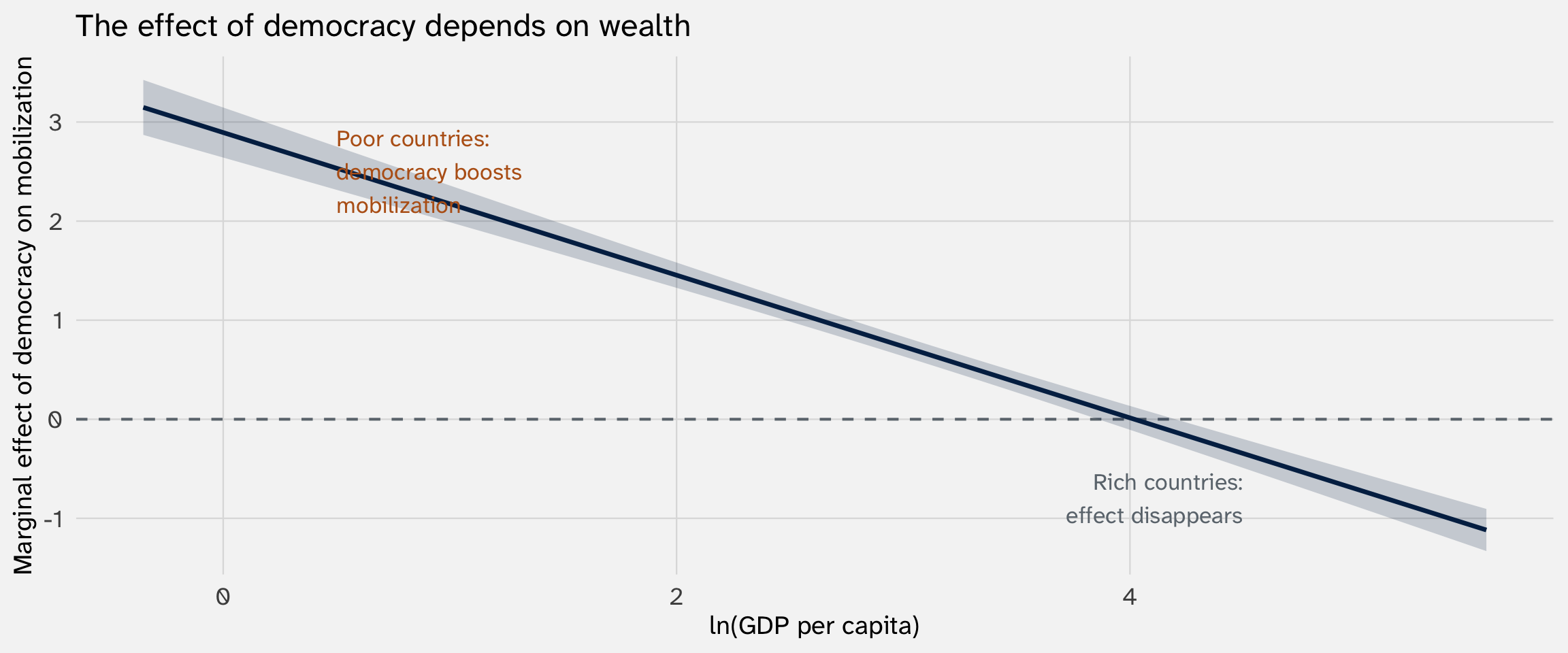
\(\hat{\beta}_3 < 0\): the effect of democracy on mobilization decreases as countries get richer
The marginal effect of democracy
\[\frac{\partial \text{mobilization}}{\partial \text{democracy}} = \beta_1 + \beta_3 \cdot \ln(\text{gdppc})\]
| GDP level | ln(GDP pc) | ≈ GDP pc ($) | Marginal effect |
|---|---|---|---|
| 25th pctile | 1.49 | 4 | 1.82 |
| Median | 2.34 | 10 | 1.21 |
| 75th pctile | 3.29 | 27 | 0.52 |
In poor countries, a one-unit increase in democracy is associated with a large increase in mobilization. In rich countries, the effect is much weaker or even negative
Marginal effects plot
The linear interaction assumption
The model \(Y = \beta_0 + \beta_1 X + \beta_2 Z + \beta_3 XZ\) assumes the marginal effect changes linearly with \(Z\):
\[\frac{\partial Y}{\partial X} = \beta_1 + \beta_3 Z\]
This is a strong assumption. The true interaction could be:
- Nonlinear: the effect changes slowly at first, then rapidly
- Threshold-based: the effect only kicks in above some value of \(Z\)
- Non-monotonic: the effect increases, then decreases
The standard interaction model can’t capture any of these
The interflex package (Hainmueller, Mummolo, and Xu 2019) estimates interaction effects nonparametrically, letting the data reveal the shape
Beyond the linear interaction
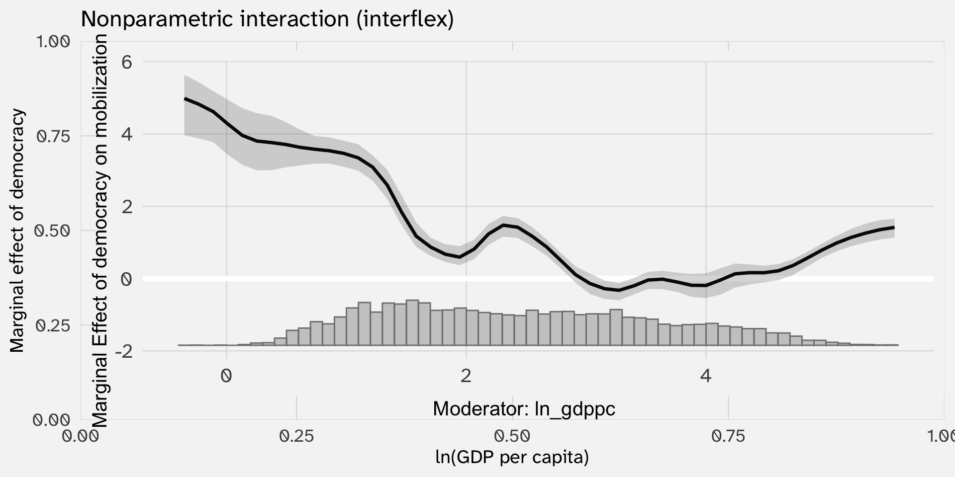
Compare this to the linear interaction—similar here, but not always
Logarithmic transformations
When theory says each additional unit matters less
- Log(X)
- Log(Y)
- log-log
Diminishing returns: A working example
Question Does economic growth improve life expectancy?
Premise 1 In very poor countries, each additional dollar buys transformative goods (clean water, basic healthcare, nutrition)
Premise 2 In wealthy countries, additional dollars go to goods with smaller health payoffs (consumer goods, cars)
Expectation Life expectancy should increase with GDP, but at a decreasing rate — diminishing returns
This is a commitment to a specific shape: each additional unit of \(X\) matters less than the last
Logging \(X\) encodes this
The data: GDP and life expectancy
| country | continent | gdp_10k | lifeExp |
|---|---|---|---|
| Afghanistan | Asia | 0.10 | 43.83 |
| Albania | Europe | 0.59 | 76.42 |
| Algeria | Africa | 0.62 | 72.30 |
| Angola | Africa | 0.48 | 42.73 |
| Argentina | Americas | 1.28 | 75.32 |
| Australia | Oceania | 3.44 | 81.24 |
Outcome lifeExp — life expectancy at birth (years)
Treatment gdp_10k — GDP per capita in $10,000s
The log(\(X\)) specification
Wrap the predictor in \(\ln()\):
\[\text{lifeExp}_i = \beta_0 + \beta_1 \cdot \ln(\text{gdp\_10k}_i) + \varepsilon_i\]
This is still OLS! We are just transforming the predictor before fitting
What is the effect of GDP on life expectancy?
| Log-level | |
|---|---|
| + p < 0.1, * p < 0.05, ** p < 0.01, *** p < 0.001 | |
| Intercept | 71.290*** |
| (0.653) | |
| ln(GDP per capita, $10k) | 7.203*** |
| (0.442) | |
| Num.Obs. | 142 |
| R2 | 0.654 |
\(\hat{\beta}_1 \approx 7.2\) — but a one-unit increase in \(\ln(\text{GDP})\) is hard to think about
Like the quadratic, we need calculus to understand what the coefficient really means
The effect depends on where you are
Write out the model and take the derivative with respect to GDP:
\[\frac{\partial}{\partial X} \left[\beta_0 + \beta_1 \cdot \ln(X) \right]\]
Apply the rule \(\frac{\text{d}}{\text{d}X} \ln(X) = \frac{1}{X}\) to each term:
\[= \underbrace{0}_{\text{constant}} + \underbrace{\beta_1 \cdot \frac{1}{X}}_{\text{log rule}}\]
\[\boxed{\frac{\partial Y}{\partial X} = \frac{\beta_1}{X}}\]
The marginal effect shrinks as GDP grows
\[\frac{\partial \text{lifeExp}}{\partial \text{gdp\_10k}} = \frac{7.2}{\text{gdp\_10k}}\]
| GDP per capita | Years per extra $1,000 |
|---|---|
| $1,000 | 7.20 |
| $5,000 | 1.44 |
| $10,000 | 0.72 |
| $40,000 | 0.18 |
Same logic as the quadratic table — plug in different values of \(X\) to see how the effect changes
Predicted life expectancy across GDP levels
Same workflow: crossing() → augment() → plot
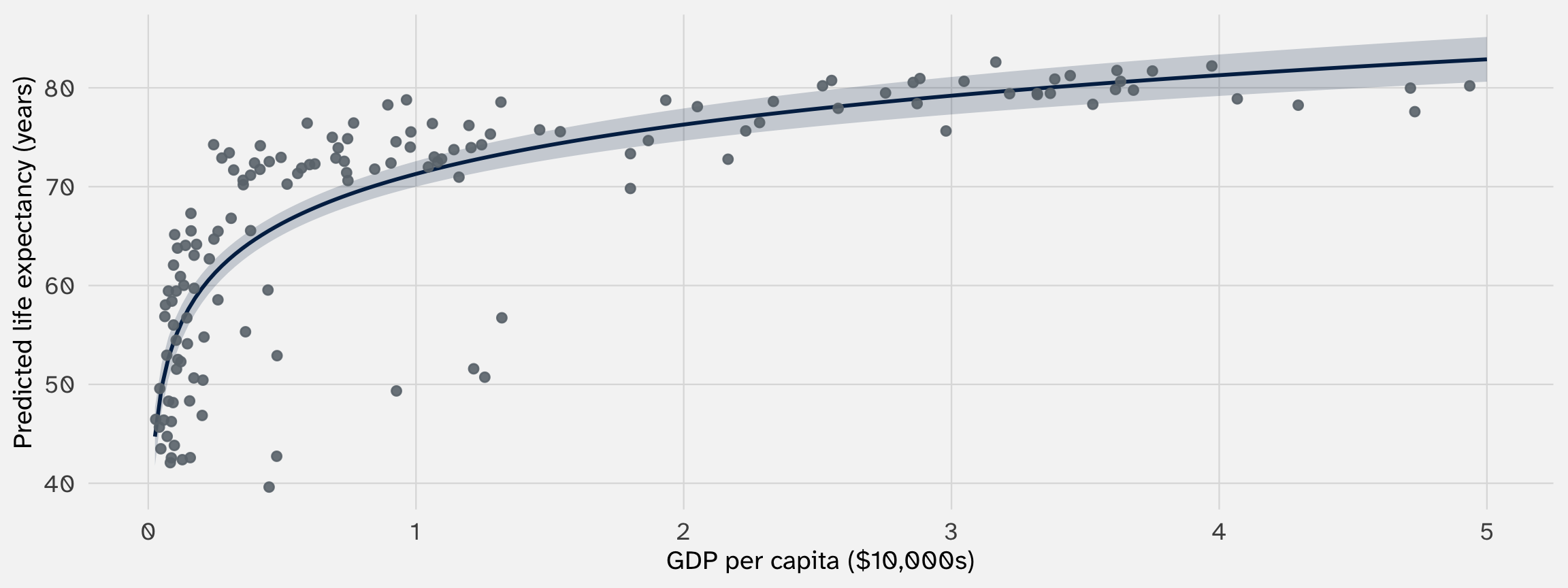
The curve flattens as GDP grows — diminishing returns, encoded by the log
The marginal effect of GDP (log \(X\))
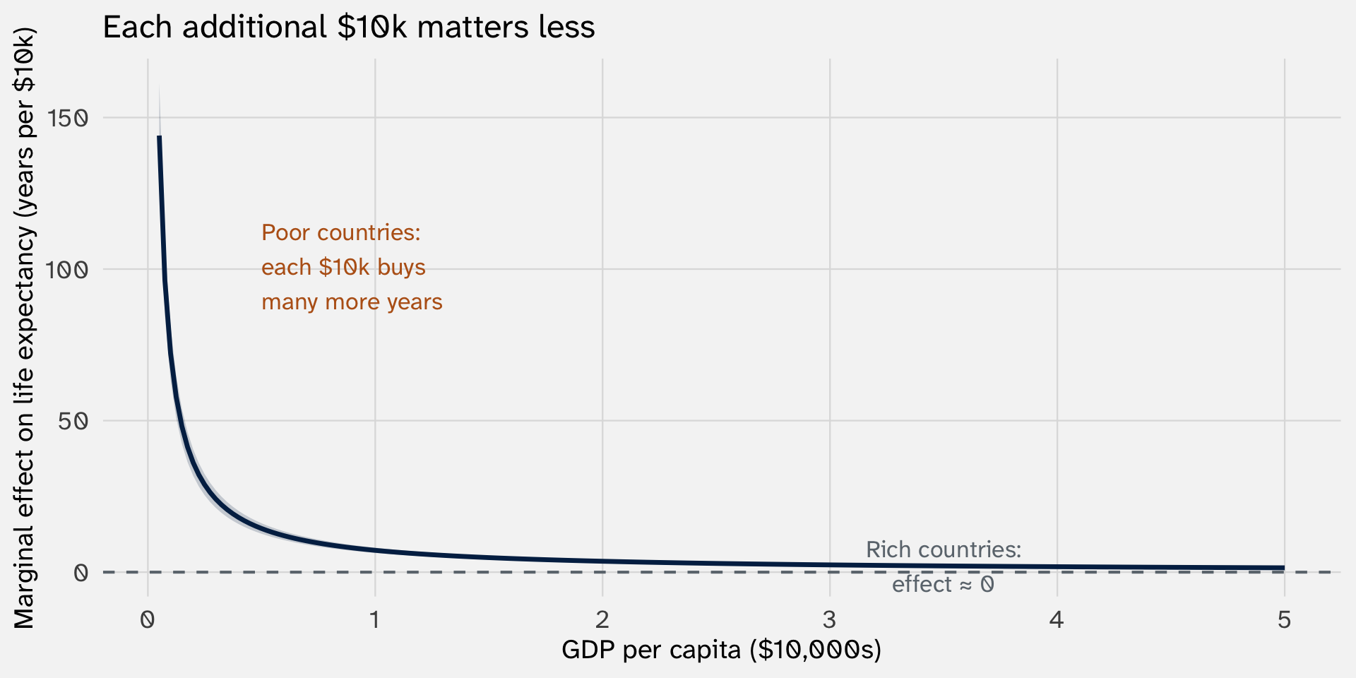
The ME is always positive but shrinking — unlike the quadratic, which crossed zero at the peak
Why slopes()?
We’ll use {marginaleffects} more as class advances, but we need it to get the standard errors for the confidence bounds
Proportional effects: A working example
Question Does a larger economy lead to more exports?
Premise 1 A country going from $1,000 to $2,000 in exports has doubled its trade
Premise 2 A country going from $1,000,000 to $1,001,000 has barely changed — same absolute increase, very different meaning
Expectation The effect of GDP on exports should be proportional — bigger economies see bigger absolute gains
Logging \(Y\) encodes this: the effect of \(X\) on \(Y\) is measured in proportions, not levels
Common for: trade volumes, military spending, population, wages — variables where ratios matter more than differences
The data: international trade
| country | exports | gdp_trillion |
|---|---|---|
| China | 1969662.9 | 15.41 |
| United States of America | 1277486.2 | 17.30 |
| Japan | 769772.7 | 4.87 |
| Netherlands | 568710.1 | 0.80 |
| France | 512743.7 | 2.54 |
| South Korea | 466376.6 | 1.73 |
Outcome exports — total exports in millions of current dollars
Treatment gdp_trillion — GDP in trillions of dollars
The log(\(Y\)) specification
Wrap the outcome in \(\ln()\):
\[\ln(\text{exports}_i) = \beta_0 + \beta_1 \cdot \text{gdp\_trillion}_i + \varepsilon_i\]
What is the effect of GDP on exports?
| Log-level | |
|---|---|
| + p < 0.1, * p < 0.05, ** p < 0.01, *** p < 0.001 | |
| Intercept | 8.640*** |
| (0.178) | |
| GDP (trillions) | 0.582*** |
| (0.091) | |
| Num.Obs. | 176 |
| R2 | 0.189 |
\(\hat{\beta}_1\) looks small — but remember, the outcome is on the log scale
The effect grows with \(Y\)
Start with the model: \(\ln(Y) = \beta_0 + \beta_1 X\)
Exponentiate both sides to undo the log and get \(Y\) by itself:
\[Y = e^{\beta_0 + \beta_1 X}\]
Now take the derivative. The rule for \(e^{f(X)}\) is \(e^{f(X)} \cdot f'(X)\):
\[\frac{\partial Y}{\partial X} = \underbrace{e^{\beta_0 + \beta_1 X}}_{\text{that's just } Y} \cdot \underbrace{\beta_1}_{f'(X)}\]
\[\boxed{\frac{\partial Y}{\partial X} = \beta_1 \cdot Y}\]
The effect of \(X\) on \(Y\) is proportional to the current level of \(Y\) — the opposite of log(\(X\)), where the effect shrank
Predicted exports across GDP levels
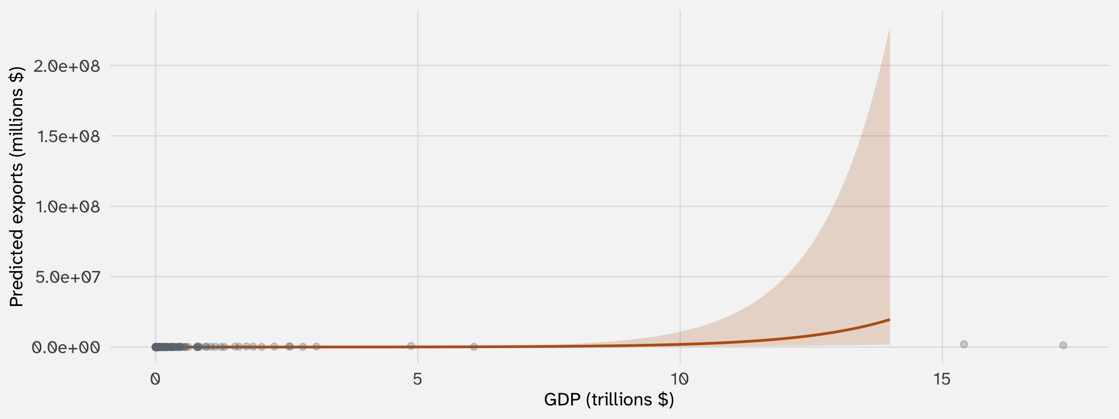
The curve accelerates — each additional trillion of GDP produces proportionally more exports, not a fixed increment
Percentage growth: A working example
Question Do exports scale proportionally with GDP?
Premise 1 What matters is not absolute dollars of GDP, but percentage growth — a 10% larger economy should mean roughly 10% more exports
Premise 2 This should hold for Lesotho ($2B) and the US ($15T) alike — the ratio is what matters, on both sides
Expectation A 1% increase in GDP → a fixed % increase in exports, regardless of the country’s size
Log(\(Y\)) asked: “what does adding $1 trillion of GDP do?” Log-log asks: “what does doubling GDP do?” — the question itself is proportional
This is the foundation of the gravity model, the workhorse of international trade
The data (same trade data)
| country | exports | gdp_trillion | pop_millions |
|---|---|---|---|
| China | 1969662.9 | 15.41 | 1283.7 |
| United States of America | 1277486.2 | 17.30 | 300.8 |
| Japan | 769772.7 | 4.87 | 122.5 |
| Netherlands | 568710.1 | 0.80 | 16.1 |
| France | 512743.7 | 2.54 | 61.9 |
| South Korea | 466376.6 | 1.73 | 46.8 |
Outcome exports — total exports in millions of current dollars
Treatment gdp_trillion — GDP in trillions of dollars
The log-log specification
Log both sides:
\[\ln(\text{exports}_i) = \beta_0 + \beta_1 \cdot \ln(\text{gdp\_trillion}_i) + \varepsilon_i\]
What is the elasticity of exports?
| Log-log | |
|---|---|
| + p < 0.1, * p < 0.05, ** p < 0.01, *** p < 0.001 | |
| Intercept | 11.837*** |
| (0.116) | |
| ln(GDP, trillions) | 1.073*** |
| (0.034) | |
| Num.Obs. | 176 |
| R2 | 0.854 |
\(\hat{\beta}_1 \approx 1.07\) — but what does this number mean?
The calculus: a ratio of percentage changes
Start with the model: \(\ln(Y) = \beta_0 + \beta_1 \ln(X)\)
Exponentiate both sides, using the rule \(e^{a + b} = e^a \cdot e^b\):
\[Y = e^{\beta_0} \cdot e^{\beta_1 \ln(X)}\]
Use the identity \(e^{c \cdot \ln(X)} = X^c\) (log and exp cancel, leaving the power):
\[Y = \underbrace{e^{\beta_0}}_{\text{constant}} \cdot X^{\beta_1}\]
This is a power function — we can differentiate with the power rule
The calculus (cont.)
\[Y = e^{\beta_0} \cdot X^{\beta_1}\]
Differentiate with the power rule:
\[\frac{\partial Y}{\partial X} = e^{\beta_0} \cdot \beta_1 \cdot X^{\beta_1 - 1} = \beta_1 \cdot \frac{\overbrace{e^{\beta_0} \cdot X^{\beta_1}}^{= Y}}{X}\]
\[\boxed{\frac{\partial Y}{\partial X} = \beta_1 \cdot \frac{Y}{X}}\]
Divide both sides by \(Y/X\) and the units cancel: \(\quad \dfrac{\partial Y / Y}{\partial X / X} = \beta_1\)
\(\beta_1\) is the % change in \(Y\) per 1% change in \(X\) — an elasticity
Predicted exports (log-log)
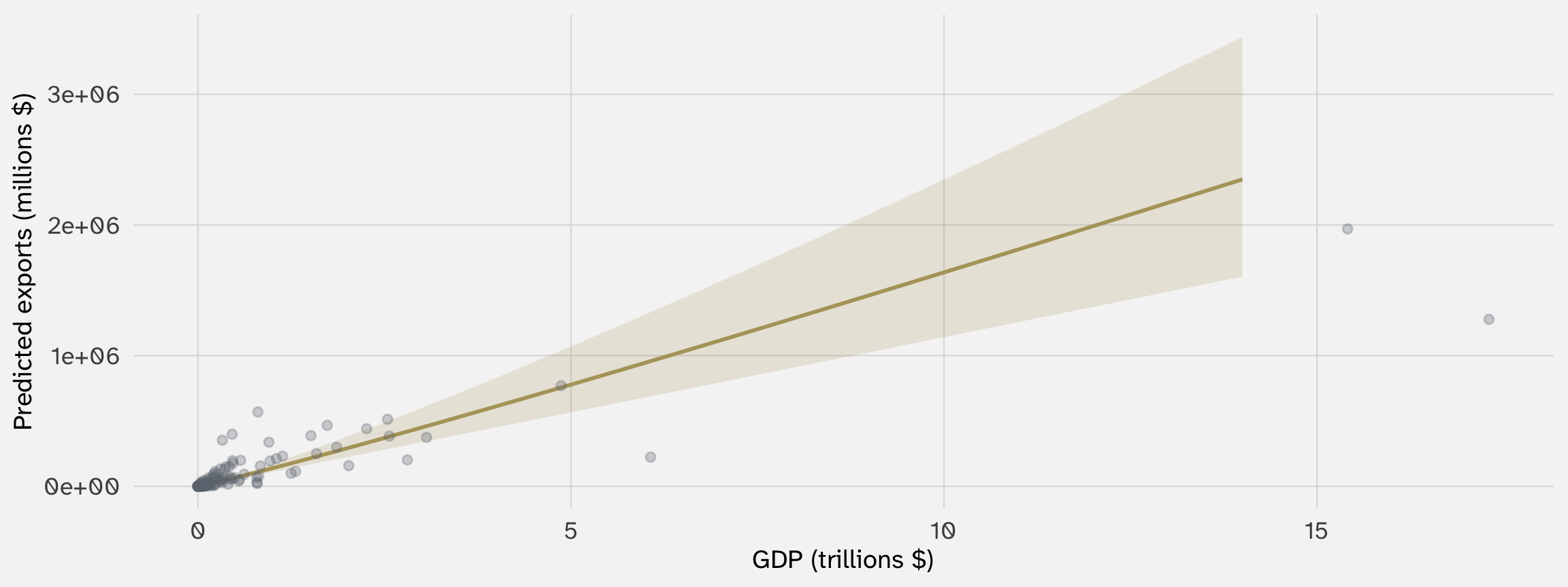
\(\hat{\beta}_1 \approx 1.07\): a 1% increase in GDP → a 1.07% increase in exports — almost perfectly proportional
Three theoretical commitments, three shapes
Each log specification encodes a different claim about the data-generating process:
| Transform | Theoretical commitment | Shape of ME |
|---|---|---|
| \(Y = \beta_0 + \beta_1 \ln X\) | Diminishing returns: each unit of \(X\) matters less | ME \(= \beta_1 / X\) (falls) |
| \(\ln Y = \beta_0 + \beta_1 X\) | Proportional scaling: same \(\Delta X\) has bigger effect at higher \(Y\) | ME \(= \beta_1 \cdot Y\) (rises) |
| \(\ln Y = \beta_0 + \beta_1 \ln X\) | Elasticity: % changes drive % changes | ME \(= \beta_1 \cdot Y/X\) (constant %) |
The choice between them is theoretical — which shape does your theory predict?
Reference: interpretation shorthands
| Model | Equation | Shorthand for \(\hat{\beta}_1\) |
|---|---|---|
| Level-level | \(Y = \beta_0 + \beta_1 X\) | 1-unit \(\uparrow\) in \(X\) → \(\beta_1\) unit \(\uparrow\) in \(Y\) |
| Level-log | \(Y = \beta_0 + \beta_1 \ln(X)\) | 1% \(\uparrow\) in \(X\) → \(\beta_1 / 100\) unit \(\uparrow\) in \(Y\) |
| Log-level | \(\ln(Y) = \beta_0 + \beta_1 X\) | 1-unit \(\uparrow\) in \(X\) → \(\beta_1 \times 100\)% \(\uparrow\) in \(Y\) |
| Log-log | \(\ln(Y) = \beta_0 + \beta_1 \ln(X)\) | 1% \(\uparrow\) in \(X\) → \(\beta_1\)% \(\uparrow\) in \(Y\) (elasticity) |
These are useful shorthands, but the marginal effects plot is always more informative
Can the data tell us what to do?
- Can we just plot it?
- Can we look at model fit?
- Can we look at residuals?
Why not always let the data choose the shape?
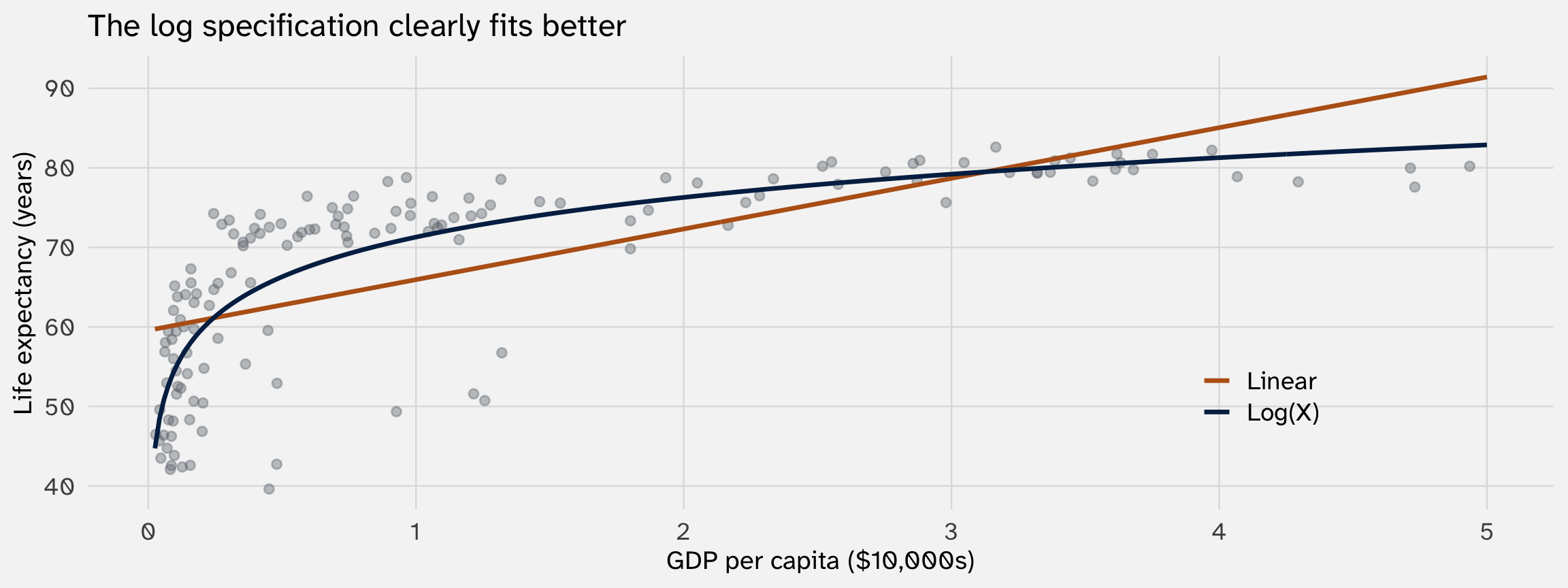
It’s obvious that log(\(X\)) fits better. So why not just try both and pick the winner?
The problem with letting the data decide
You should look at your data. Plotting before modeling is good practice
But there are limits:
1. Multivariate relationships are hard to see. With 5+ controls, the partial relationship between \(X\) and \(Y\) isn’t visible in a raw scatterplot. You need residual plots, which already assume a model
2. Theory should guide specification. The “more murder in the middle” hypothesis predicts a quadratic—we aren’t just curve-fitting. Without theory, you risk overfitting patterns that don’t replicate
3. Researcher degrees of freedom. If you try linear, quadratic, cubic, log, sqrt… and pick the best-looking one, you are running a specification search. The more forms you try, the more likely you find something by chance
Takeaway Always look at your data—but there’s (probably?) no theory-free way to fit a model
Higher-degree polynomials chase noise
A polynomial with enough terms can bend to fit any pattern—including noise
Let’s test this: draw two independent random subsamples and fit a quadratic vs. a degree-6 polynomial to each
If both models capture the signal, they should tell the same story in both samples
Do the results replicate?
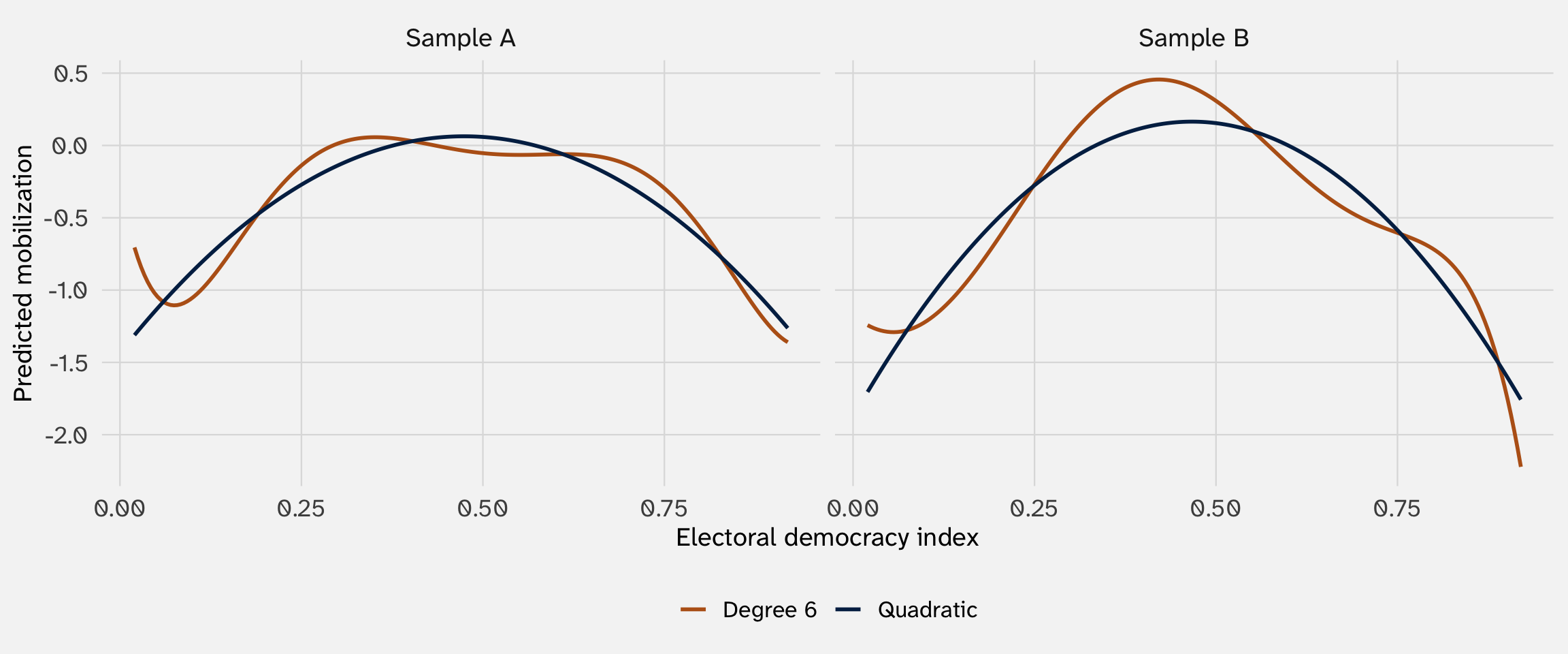
The quadratic tells the same story in both samples. The degree-6 polynomial tells different stories—its wiggles are artifacts of whichever 300 country-years happened to land in each subsample
The complexity–power tradeoff
Every transformation adds parameters to estimate—and parameters cost statistical power
| Specification | New parameters | What it costs |
|---|---|---|
| \(X\) (linear) | 1 | — |
| \(X + X^2\) (quadratic) | 2 | Modest |
| \(X \times Z\) (interaction) | 1 more | Splits data by \(Z\) |
| \(X \times Z + X^2 \times Z\) | 2 more | Separate curves per group |
The core issue: a main effect of democracy uses all 11,000 country-years. An interaction with region slices that into ~1,000 per region. Each subgroup estimate is noisier, confidence intervals widen
The tradeoff: richer specifications ask richer questions (“does the inverted-U differ across regions?”) but you pay with precision. With small samples, real heterogeneity may not reach significance
Just because you can interact and square everything doesn’t mean your data can support it
How bad is the power loss? Worse than you think
Gelman and Carlin (2014) show this with a simple example:
Suppose a study has 80% power for a main effect. How much power does it have for an interaction?
SE of a main effect: \(\;\text{se}(\bar{y}_1 - \bar{y}_2) = \frac{2\sigma}{\sqrt{N}}\)
SE of an interaction (difference in differences): \(\;\text{se}\left[(\bar{y}_1 - \bar{y}_2) - (\bar{y}_3 - \bar{y}_4)\right] = \frac{4\sigma}{\sqrt{N}}\)
The interaction SE is 2\(\times\) the main effect SE
Two penalties compound
Two things work against you when estimating an interaction:
- The SE is 2\(\times\) bigger (we just showed this: \(4\sigma/\sqrt{N}\) vs. \(2\sigma/\sqrt{N}\))
- The effect is usually smaller: an interaction asks “does the effect differ across groups?” The difference between two effects is almost always smaller than either effect alone. Gelman and Carlin (2014) suggest half the main effect as a reasonable rule of thumb
Smaller effect \(\div\) bigger SE: the z-score is \(\frac{1}{2} \div 2 = \frac{1}{4}\) of the main effect’s. 80% power for the main effect → roughly 10% power for the interaction
You need 16\(\times\) the sample size to estimate an interaction as to estimate a main effect
Recall: the z-score
\(z = \frac{\hat{\beta}}{\text{SE}(\hat{\beta})}\) — how many standard errors the estimate is from zero. Larger z → more evidence against the null. We reject at \(|z| > 1.96\) (95% level).
It gets worse: the winner’s curse
10% power doesn’t just mean you’ll usually miss the interaction. It means the rare “wins” are wildly inflated
The true z-score is 0.7, but the average z-score among significant results is 2.4 — over 3\(\times\) the true value
This is the winner’s curse: when power is low, statistical significance selects for overestimates
What about \(R^2\)?
Another tempting diagnostic: why not pick the model that “explains” the data better?
\[R^2 = 1 - \frac{\sum (Y_i - \hat{Y}_i)^2}{\sum (Y_i - \bar{Y})^2}\]
\(R^2 = 0\): the model explains nothing beyond the mean of \(Y\)
\(R^2 = 1\): the model predicts every observation perfectly
Surely a higher \(R^2\) means a better model?
Low \(R^2\) can still mean a correct estimate
Simulate a randomized experiment where the true effect of treatment = 5
| Experiment | |
|---|---|
| + p < 0.1, * p < 0.05, ** p < 0.01, *** p < 0.001 | |
| Intercept | 18.969*** |
| (1.887) | |
| Treatment | 5.834* |
| (2.669) | |
| R2 | 0.010 |
\(R^2 \approx 0.01\) — the model explains almost nothing. But the treatment effect estimate is spot on (\(\hat{\beta} \approx 5\), the true value)
The lesson: \(R^2\) measures prediction, not identification
Low \(R^2\) means lots of unexplained variation in \(Y\) — history, personality, shocks, luck
But the treatment effect can still be correctly estimated if the model is well-specified. The goal of most social science is to identify a relationship, not predict every data point
When is \(R^2\) useful?
Fit matters for prediction: how well can I forecast \(Y\) for new observations? It matters less for causal inference, where the goal is getting \(\hat{\beta}\) right, not \(\hat{Y}\) right. But this is debated!
Next week
- So far we’ve assumed \(Y\) is continuous and used OLS
- But many outcomes in political science are binary: war or peace, vote or abstain, win or lose
- Next week: logistic regression → our first MLE-based model