| protestant | oppose_aca | wall | conceal | oppose_minwage | age | sex | newsint |
|---|---|---|---|---|---|---|---|
| Non-Protestant | 1 | 1 | 0 | 1 | 54 | Male | Most of the time |
| Protestant | 1 | 0 | 0 | 0 | 65 | Female | Most of the time |
| Protestant | 1 | 0 | 0 | 0 | 74 | Female | Most of the time |
| Non-Protestant | 0 | 0 | 0 | 0 | 58 | Female | Some of the time |
| Non-Protestant | 1 | 0 | 1 | 0 | 53 | Male | Only now and then |
| Protestant | 0 | 1 | 1 | 1 | 59 | Male | Most of the time |
Binary Outcomes and the Logit Model
POL 213 · Week 3
Juan F. Tellez
University of California, Davis
April 15, 2026
Housekeeping
- PS1 grades
- PS2
- Group projects
Logit
The two wolves within political science
Recall from week 1: two traditions pull in different directions
Economics
Causal inference, estimation of effects (Angrist and Pischke (2009))
“Use the simplest model that identifies the effect”
Statistics
Modeling the data-generating process (Gelman, Hill, and Vehtari (2020))
“Use models that match the structure of your data”
Today’s topic is contentious between these camps
The logit wars



Why a war?
Two questions, two emphases
Econometrics / design-based inference
Q What is the effect of \(X\) on \(Y\)?
\[Y_i = \alpha + \beta \, X_i + \varepsilon_i\]
The object of interest is \(\hat{\beta}\) — a single number for how \(Y\) responds to \(X\)
The model is a tool. Functional form is secondary; what matters is that \(\hat{\beta}\) recovers the causal effect under a good research design
Statistics / model-based inference
Q How is \(Y\) generated given \(X\)?
\[\mathbb{E}[Y_i \mid X_i] \;=\; f(X_i; \boldsymbol{\theta})\]
The object of interest is \(f(\cdot)\) — the full function mapping \(X\) to the expected value of \(Y\)
The model is the answer. Coefficients are features of \(f\); interpretation depends on the whole specification
Economists want a clean \(\hat{\beta}\). Statisticians want an \(f\) that faithfully captures the data-generating process
I am speaking loosely
Economists and statisticians vary a lot among themselves on these questions; I am using these disciplines as useful metaphors
How logit is traditionally motivated
The standard story you’ll see in MLE:
| Outcome type | Example | Model |
|---|---|---|
| Continuous | Vote share, GDP growth | OLS |
| Binary | Vote turnout, war onset | Logit / Probit |
| Count | # protests, # coups in a year | Poisson / NB |
| Ordered categories | Strongly disagree … strongly agree | Ordered logit |
| Unordered categories | Party choice (Dem / Rep / Indep / Green) | Multinomial logit |
| Time to event | Regime duration, conflict duration | Survival / Cox |
But notice: this is a statistics view — match the model to the structure of \(Y\)
The economics view is more skeptical: if you want the average treatment effect (ATE), OLS on a binary \(Y\) may be just fine
Treatment effects with a binary outcome
A working example
Question Does religion shape one’s politics?
Premise 1 Some religious traditions have become increasingly politicized
Premise 2 Regular exposure to political messaging from the pulpit can shape members’ views
Expectation Belonging to a conservative religious tradition → more conservative political views
The data: 2020 Cooperative Election Study
Four binary outcomes (policy support), one binary treatment (Protestant), three controls (age, sex, news interest)
Goal estimate the effect of being Protestant on each policy preference, controlling for age, sex, and news interest
A note on measurement
Ideally we’d look specifically at evangelical Christians — the group where the politicization story is strongest. But the CES doesn’t ask a direct evangelical-identity question, so I use Protestant as a rough proxy. Sorry!
Estimating effects by hand
Average differences between groups
The simplest estimator
How do we estimate the effect of a binary treatment, without any model?
Compare averages across groups → the classic difference-in-means estimator:
\[\hat{\tau} = \bar{Y}_{\text{Protestant}} - \bar{Y}_{\text{Non-Protestant}}\]
When \(Y\) is binary, the mean is just a proportion — the share of 1s in the group:
\[\bar{Y} \;=\; \frac{1}{n} \sum_{i} Y_i \;=\; \frac{\text{number of 1s}}{n} \;=\; \hat{p}\]
So the difference-in-means is a difference in probabilities of supporting the policy → same estimator, different name
Average support, by group
# group means are just proportions when Y is 0/1
# all four outcomes are coded so that 1 = more conservative position
group_means = bot_clean |>
  group_by(protestant) |>
  summarize(
    `Oppose ACA`      = mean(oppose_aca),
    `Support wall`    = mean(wall),
    `Support conceal` = mean(conceal),
    `Oppose min wage` = mean(oppose_minwage),
    `% of sample`     = 100 * n() / nrow(bot_clean)
)| protestant | Oppose ACA | Support wall | Support conceal | Oppose min wage | % of sample |
|---|---|---|---|---|---|
| Non-Protestant | 0.638 | 0.330 | 0.323 | 0.263 | 68.372 |
| Protestant | 0.489 | 0.524 | 0.433 | 0.425 | 31.628 |
The by-hand effects
| Outcome | Non-Protestant | Protestant | Difference |
|---|---|---|---|
| Oppose ACA | 0.638 | 0.489 | -0.150 |
| Support wall | 0.330 | 0.524 | 0.194 |
| Support conceal | 0.323 | 0.433 | 0.110 |
| Oppose min wage | 0.263 | 0.425 | 0.163 |
Three differences are positive → Protestants more conservative, as expected
One (ACA) is negative → Protestants less likely to oppose ACA
Standard errors of the differences
How precise are these differences?
Formula (two independent proportions):
\[\text{SE}(\hat{p}_1 - \hat{p}_0) \; = \; \sqrt{\frac{\hat{p}_1 \, (1 - \hat{p}_1)}{n_1} + \frac{\hat{p}_0 \, (1 - \hat{p}_0)}{n_0}}\]
# group sizes
n_P  = sum(bot_clean$protestant == "Protestant")
n_NP = sum(bot_clean$protestant == "Non-Protestant")

# SE of the difference in proportions, plus z-statistic
by_hand_se = by_hand |>
  mutate(
    SE = sqrt(Protestant * (1 - Protestant) / n_P +
              `Non-Protestant` * (1 - `Non-Protestant`) / n_NP),
    z  = Difference / SE
  )
The by-hand effects (with uncertainty)
| Outcome | Non-Protestant | Protestant | Difference | SE | z |
|---|---|---|---|---|---|
| Oppose ACA | 0.638 | 0.489 | -0.150 | 0.00431 | -34.8 |
| Support wall | 0.330 | 0.524 | 0.194 | 0.00428 | 45.3 |
| Support conceal | 0.323 | 0.433 | 0.110 | 0.00425 | 25.8 |
| Oppose min wage | 0.263 | 0.425 | 0.163 | 0.00417 | 39.0 |
Notice the SEs are all nearly identical (≈ 0.0043). Not an accident — the Bernoulli SE
\[\text{SE}(\hat{p}) \;=\; \sqrt{\frac{p\,(1 - p)}{n}}\]
is largest at \(p = 0.5\) and shrinks toward 0 as \(p\) moves toward 0 or 1. With all four proportions in [0.26, 0.64], we’re sitting near the peak → the SE barely changes between outcomes
With \(n \approx 60{,}000\), even the smallest effect (\(\approx 11\) pts on concealed carry) has \(|z| \approx 26\) — all four differences have tiny p-values
Regression recovers the same estimate
An OLS regression of \(Y\) on a binary treatment gets you the same result:
\[Y_i = \beta_0 + \beta_1 \cdot \mathbf{1}(\text{Protestant}_i) + \varepsilon_i\]
- \(\beta_0\) = mean of \(Y\) among Non-Protestants
- \(\beta_1\) = difference in means (Protestant − Non-Protestant)
By hand
| Outcome | Difference | SE |
|---|---|---|
| Oppose ACA | -0.14976 | 0.00431 |
From lm()
| term | estimate | std.error |
|---|---|---|
| protestantProtestant | -0.14976 | 0.00425 |
Coefficient matches exactly
The SE is close but not identical → classical OLS assumes homoskedasticity: but binary \(Y\) is always heteroskedastic
Brief aside: Heteroskedasticity
The standard error of the OLS coefficient:
\[\text{SE}(\hat{\beta}_1) \;=\; \sqrt{\frac{\sigma^2_{\varepsilon}}{\sum_i (X_i - \bar{X})^2}}\]
Numerator: \(\sigma^2_{\varepsilon}\) — residual variance, how much \(Y\) scatters around the fitted line (the unexplained part of \(Y\))
Denominator: \(\sum_i (X_i - \bar{X})^2\) — how spread out the predictor is across units
With multiple predictors
The denominator becomes the residual variance of \(X_j\) — the variation in \(X_j\) not already explained by the other predictors:
\[\text{SE}(\hat{\beta}_j) \;=\; \sqrt{\frac{\sigma^2_{\varepsilon}}{\sum_i (X_{ij} - \bar{X}_j)^2 \,\cdot\, (1 - R^2_j)}}\]
Computing the numerator with broom
Square the residuals, sum them, divide by \(n - k\) degrees of freedom:
# A tibble: 1 × 3
     SSR    df sigma2
   <dbl> <dbl>  <dbl>
1 14386. 60726  0.237
→ \(\sigma^2_{\varepsilon} = 0.237\)
Plug in (the denominator is 13,132 for our binary treatment):
\[\text{SE}(\hat{\beta}_1) \;=\; \sqrt{\frac{0.237}{13,132}} \;=\; 0.00425\]
matches tidy(mod_aca) exactly
# A tibble: 1 × 5
  term                 estimate std.error statistic   p.value
  <chr>                   <dbl>     <dbl>     <dbl>     <dbl>
1 protestantProtestant   -0.150   0.00425     -35.3 1.28e-269
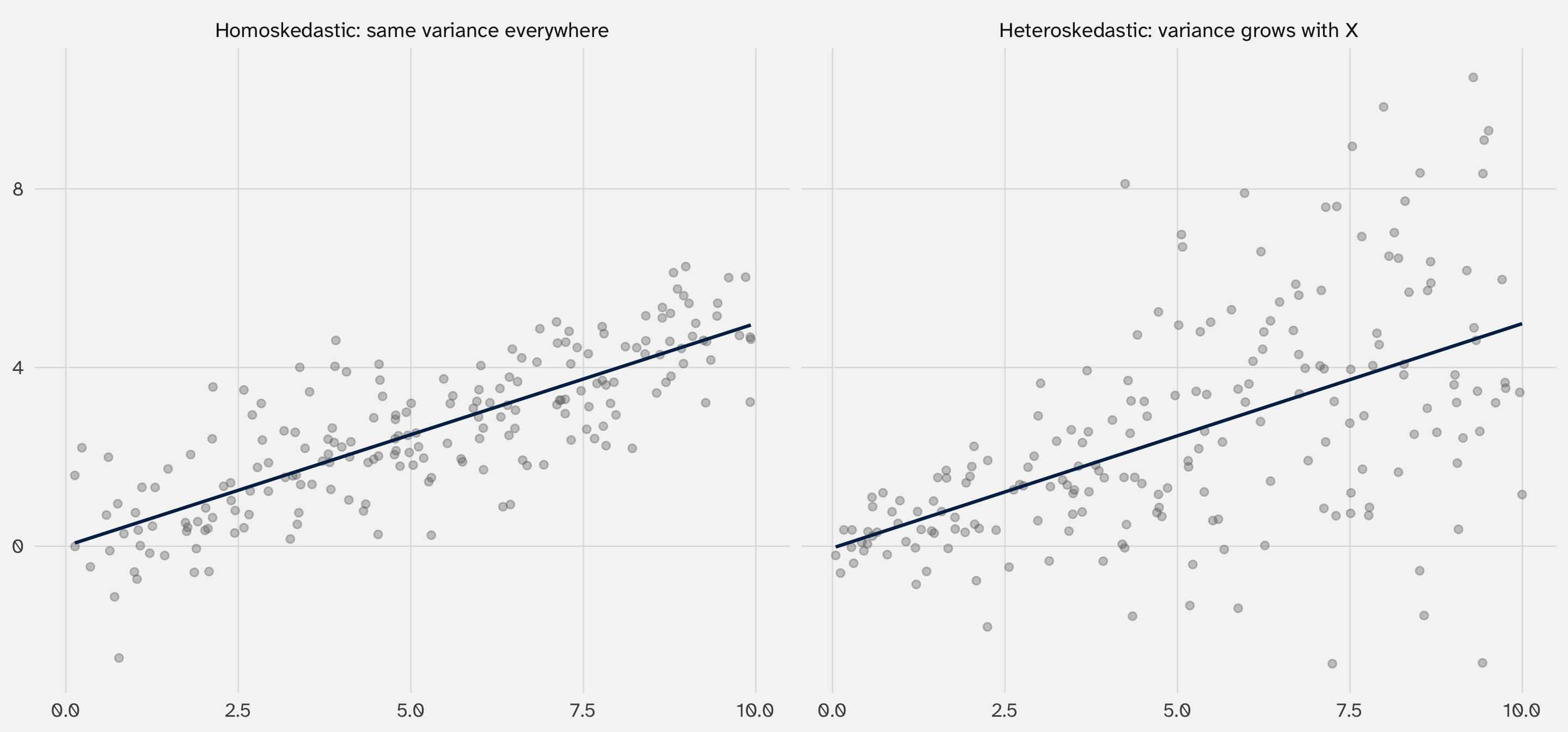
Homoskedastic vs heteroskedastic
Homo-skedastic (what OLS assumes): every observation has the same residual variance
Every observation is \(\approx\) easy to predict. A 20-year-old and a 70-year-old are equally predictable (or equally noisy) given their \(X\).
Hetero-skedastic: residual variance differs across observations → using one number is wrong
Some observations are easier to predict than others. Classic real-world examples: income → spending (wealthy people have more variable spending)
binary outcomes are inherently heteroskedastic
Classic funnel plots
Why binary \(Y\) is always heteroskedastic
For a Bernoulli outcome, the residual variance is pinned down by the group mean:
\[\text{Var}(Y \mid X) \;=\; p(X) \, (1 - p(X))\]
Since \(p(X)\) differs across groups (the whole point of the regression), residual variance must differ too
Our ACA model, by group:
| protestant | p̂ | Var(Y | group) |
|---|---|---|
| Non-Protestant | 0.638 | 0.231 |
| Protestant | 0.489 | 0.250 |
Classical OLS averages these into one number (≈ 0.237) and uses it for everyone → SE off by a little
Robust SEs use each group’s variance separately → next slide
Robust SEs: use each group’s own variance
Instead of pooling, plug each group’s own variance into the SE formula:
\[\text{SE}_{\text{HC2}}(\hat{\beta}_1) \;=\; \sqrt{\frac{v_{\text{NP}}}{n_{\text{NP}}} + \frac{v_{\text{P}}}{n_{\text{P}}}}\]
# A tibble: 1 × 1
   SE_HC2
    <dbl>
1 0.00431
lm_robust(..., se_type = "HC2") computes robust standard errors by default:
| term | estimate | std.error |
|---|---|---|
| protestantProtestant | -0.14976 | 0.00431 |
How much does it matter?
| Method | SE |
|---|---|
Classical (lm) |
0.00425 |
HC2 robust (lm_robust) |
0.00431 |
The HC2 SE is about 1.5% larger than the classical SE on this data . . .
My recommendation: heteroskedasticity is the norm, use robust standard errors by default → very narrow edge cases (e.g., very small sample) where classical are better
That’s why the estimatr package exists: lm_robust() makes HC standard errors a one-line command instead of a manual sandwich computation
Every outcome, robust SEs
Same four models, with HC2 standard errors:
# four models, HC2-robust SEs
mods_rb = list(
  `Oppose ACA`      = lm_robust(oppose_aca     ~ protestant, data = bot_clean, se_type = "HC2"),
  `Support wall`    = lm_robust(wall           ~ protestant, data = bot_clean, se_type = "HC2"),
  `Support conceal` = lm_robust(conceal        ~ protestant, data = bot_clean, se_type = "HC2"),
  `Oppose min wage` = lm_robust(oppose_minwage ~ protestant, data = bot_clean, se_type = "HC2")
)| Oppose ACA | Support wall | Support conceal | Oppose min wage | |
|---|---|---|---|---|
| + p < 0.1, * p < 0.05, ** p < 0.01, *** p < 0.001 | ||||
| Protestant | -0.150*** | 0.194*** | 0.110*** | 0.163*** |
| (0.004) | (0.004) | (0.004) | (0.004) | |
| Intercept | 0.638*** | 0.330*** | 0.323*** | 0.263*** |
| (0.002) | (0.002) | (0.002) | (0.002) | |
| Num.Obs. | 60728 | 60728 | 60728 | 60728 |
We can use the linear probability model to estimate effects
What we just did — OLS on a binary outcome — has a name: the Linear Probability Model (LPM)
Why “probability”? When \(Y \in \{0, 1\}\), \(\mathbb{E}[Y \mid X] = \Pr(Y = 1 \mid X)\)
So every \(\beta\) in lm(Y ~ X) is the effect of \(X\) on the probability that \(Y = 1\)
Why “linear”? Because we force that probability to be a linear function of \(X\):
\[\Pr(Y = 1 \mid X) \;=\; \beta_0 + \beta_1 \, X\]
Angrist & Pischke (Angrist and Pischke 2009, ch. 3) defend the LPM: if your identification strategy is sound, OLS on a binary outcome recovers the causal effect on the probability scale — logit or probit don’t add identification power
So the LPM can recover treatment effects
📝 Activity: do it yourself
Use the affairs dataset from juanr (Fair 1978, n = 601)
Question do people with kids have affairs at different rates than people without?
Steps:
- Create a binary outcome:
had_affair - Compute the by-hand effect of
kids: group proportions, difference, and the two-sample SE - Fit the LPM with classical SE — does the coefficient match? Does the SE match?
- Fit the LPM with robust SE — now does the SE match?
- How big is the difference between classical and robust SE here?
Statisticians focus on the distribution
The economics view: LPM works if identification is sound
The statistics view: you’re still not modeling the DGP of a binary outcome
What we actually observe, one row at a time, is just 0s and 1s:
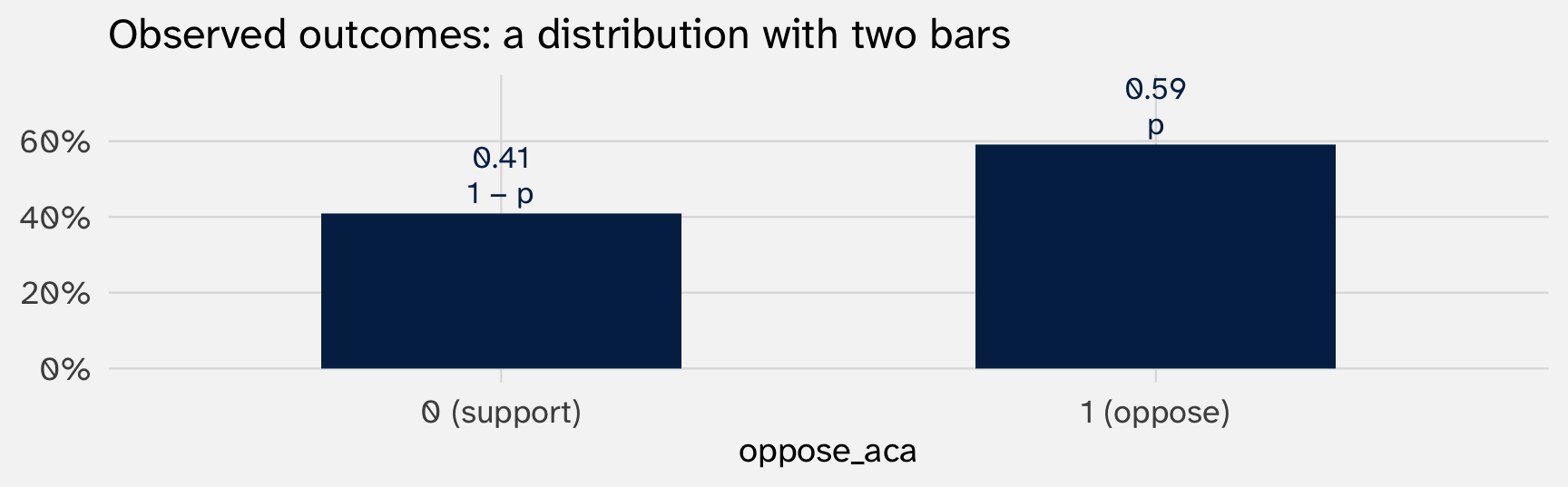
This is a Bernoulli distribution. It’s fully described by one number, \(p\) = the probability of a 1
Modeling \(p\) as a function of \(X\)
Binary outcomes are governed by a Bernoulli distribution:
\[Y_i \sim \text{Bernoulli}(p_i), \qquad p_i = \Pr(Y_i = 1 \mid X_i)\]
The statistician’s job: model \(p_i\) directly as a function of covariates
\[p_i \;=\; f(X_i; \boldsymbol{\theta})\]
One constraint: whatever \(f\) we pick, it must respect \(p \in [0, 1]\) — there’s no such thing as a probability below 0 or above 1
The LPM — a straight line — does not respect this bound. That’s where the critique begins
Why not the LPM?
Three problems with treating binary \(Y\) as if it were continuous
What’s wrong with the LPM?
1. Predictions can fall outside [0, 1]
LPM is a line — eventually it must cross 0 or 1 for some values of \(X\). Probabilities cannot
2. Constant marginal effect is implausible
LPM says \(\partial p / \partial X\) is the same at \(p = 0.5\) and at \(p = 0.95\). But probabilities have floors and ceilings → effects should shrink near the extremes
3. No model of the DGP
LPM draws a line through a cloud of 0s and 1s without any claim about how \(Y\) is generated. The statistician wants a story
(We already handled a 4th problem — heteroskedasticity — with HC2 standard errors)
LPM predictions can escape [0, 1]
Using the affairs data, regress had_affair on three controls: marriage rating, years married, and religiosity
Pull each observation’s fitted probability with broom::augment():
# A tibble: 7 × 10
  had_affair marriage_rating years_married relig .fitted .resid   .hat .sigma
       <dbl>           <int>         <dbl> <int>   <dbl>  <dbl>  <dbl>  <dbl>
1          0               5         0.75      5 -0.0175 0.0175 0.0114  0.414
2          1               5         0.75      5 -0.0175 1.02   0.0114  0.412
3          0               5         1.5       5 -0.0105 0.0105 0.0107  0.414
4          0               5         1.5       5 -0.0105 0.0105 0.0107  0.414
5          0               5         1.5       5 -0.0105 0.0105 0.0107  0.414
6          0               5         0.75      5 -0.0175 0.0175 0.0114  0.414
7          0               5         0.417     5 -0.0206 0.0206 0.0117  0.414
# ℹ 2 more variables: .cooksd <dbl>, .std.resid <dbl>
A line must eventually cross 0 or 1 — with enough predictors pulling in the same direction, the line crosses while still inside the data
Constant slopes don’t respect bounds
The LPM’s coefficient is the marginal effect: one number, same for everyone:
So a one-unit increase in marriage rating always changes Pr(affair) by the same \(-0.10\) — regardless of where the baseline sits:
| Baseline Pr | LPM effect | New Pr |
|---|---|---|
| 0.05 | -0.1 | -0.05 |
| 0.30 | -0.1 | 0.20 |
| 0.50 | -0.1 | 0.40 |
| 0.70 | -0.1 | 0.60 |
| 0.95 | -0.1 | 0.85 |
→ at baseline 0.05, the LPM predicts a new probability of −0.05 — impossible
Intuitively, effects should shrink near the floor and ceiling → you can’t fall below 0 or rise above 1
Logit: a bounded linear model
Keep the linear combination, bend the output to live in [0, 1]
What we want
Keep the machinery of linear models → still a weighted sum of predictors:
\[X\beta \;=\; \beta_0 + \beta_1 X_1 + \beta_2 X_2 + \cdots\]
But pass this linear combination through a function \(g^{-1}(\cdot)\) that squashes any real number into \([0, 1]\):
\[\Pr(Y = 1 \mid X) \;=\; g^{-1}(X\beta)\]
\(g^{-1}\) is the inverse link function (or “response function”)
We need one more thing: a function whose shape makes sense for probabilities — symmetric, monotone, with smooth floors and ceilings
The logistic function
\[\sigma(z) \;=\; \frac{1}{1 + e^{-z}}\]
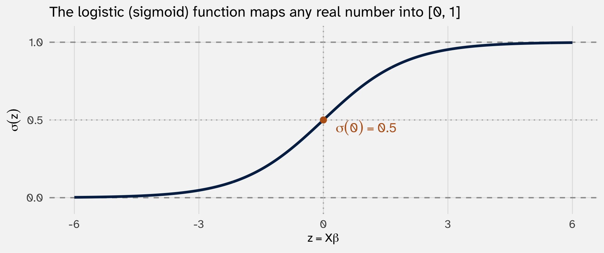
Bounded, monotone, symmetric around \(z = 0\) where \(\sigma = 0.5\). Steepest in the middle, flat at the extremes — the slope varies with \(z\)
Logit regression
Apply the logistic to \(X\beta\):
\[\Pr(Y = 1 \mid X) \;=\; \sigma(X\beta) \;=\; \frac{1}{1 + e^{-X\beta}}\]
Fit it with glm() using family = binomial() (which defaults to the logit link):
| term | estimate | std.error | statistic | p.value |
|---|---|---|---|---|
| (Intercept) | -0.7062 | 0.0104 | -67.6880 | 0 |
| protestantProtestant | 0.8034 | 0.0178 | 45.0829 | 0 |
Coefficients are in log-odds units → not directly interpretable as changes in probability
Why log-odds? And how do we read this coefficient? → next two slides
Why log-odds?
Start from the logit, letting \(P = \Pr(Y = 1 \mid X)\):
\[P \;=\; \frac{1}{1 + e^{-X\beta}}\]
Step 1 — take the reciprocal of both sides:
\[\frac{1}{P} \;=\; 1 + e^{-X\beta}\]
Step 2 — isolate the exponential (subtract 1, combine the right side):
\[e^{-X\beta} \;=\; \frac{1}{P} - 1 \;=\; \frac{1 - P}{P}\]
Step 3 — take the log and flip the sign:
\[X\beta \;=\; \log\!\left(\frac{P}{1 - P}\right)\]
The log-odds parameterization
What we just derived:
\[\underbrace{\log\frac{P}{1 - P}}_{\text{log-odds (logit) of } P} \;=\; \beta_0 + \beta_1 X_1 + \cdots\]
Why is this the natural form?
- Log-odds is unbounded (\(-\infty\) to \(+\infty\)) → matches \(X\beta\)’s range
- The sigmoid is just the inverse of the log-odds → pushes \(X\beta\) back into \([0, 1]\)
→ Each \(\beta\) is the change in log-odds for a one-unit change in \(X\). Not yet a probability (we’ll convert later)
Interpreting the Protestant effect
Our model: glm(wall ~ protestant, family = binomial) → \(\hat{\beta}_{\text{Protestant}} = 0.803\)
Way 1 — exponentiate to get an odds ratio ❌
\[e^{0.803} = 2.23\]
Protestants have 2.23× the odds of supporting the wall
I don’t like this; what does this even mean?
Generate predicted \(\widehat{Y}\)
Way 2 — convert to probabilities by setting a scenario
Build the two scenarios with crossing() (same workflow as weeks 1-2), then push them through the model with augment():
| protestant | Pr(wall) |
|---|---|
| Non-Protestant | 0.330 |
| Protestant | 0.524 |
- Non-Protestant: \(\sigma(-0.705) \;=\; \dfrac{1}{1 + e^{0.705}} \;=\; \dfrac{1}{1 + 2.024} \;=\; \mathbf{0.331}\)
- Protestant: \(\sigma(-0.705 + 0.803) \;=\; \sigma(0.098) \;=\; \dfrac{1}{1 + e^{-0.098}} \;=\; \dfrac{1}{1 + 0.907} \;=\; \mathbf{0.524}\)
So support for the wall is about 20pp higher among Protestants
Interpreting logit effects
When the model is nonlinear, the “effect of \(X\)” depends on where you are
A familiar pattern
Week 1: OLS
\[Y = \beta_0 + \beta_1 X + \varepsilon\]
Effect of \(X\) on \(Y\) is the coefficient itself — same everywhere
Tool: algebra
Week 2: Transformed OLS
\[Y = \beta_0 + \beta_1 X + \beta_2 X^2 + \varepsilon\]
Effect depends on where you are in \(X\). You chose the nonlinearity
Tools: calculus + visualization
Week 3: Logit
\[\Pr(Y = 1) = \sigma(\beta_0 + \beta_1 X)\]
Effect depends on where you are in \(X\). The model imposed the nonlinearity
Tools: calculus + visualization (same as week 2)
Week 2 you decided whether effects were nonlinear; this week nonlinearity is default
The marginal effect is not constant
In OLS: the effect of \(X\) on \(Y\) is always \(\beta_1\) — one number, same for everyone
In logit: the effect of \(X\) on \(P\) depends on where you are on the sigmoid
Remember the sigmoid’s shape:
- Steep in the middle (around \(p = 0.5\)) → a small change in \(X\) moves \(p\) a lot
- Flat at the edges (near \(p = 0\) or \(1\)) → the same change in \(X\) barely moves \(p\)
So the “effect” of \(X\) is whatever the sigmoid’s slope happens to be at your current position. Let’s compute it
Deriving \(dP/dX\)
\(X\) doesn’t move \(P\) directly — it moves \(z\), which moves \(P\):
\[X \;\longrightarrow\; z = \beta_0 + \beta_1 X \;\longrightarrow\; P = \sigma(z)\]
Step 1 — how much does \(z\) move when \(X\) moves by 1?
\[\frac{dz}{dX} \;=\; \beta_1 \qquad \text{(slope of the linear part)}\]
Step 2 — now \(z\) has moved. How much does \(P\) move per unit of \(z\)?
\[\frac{d\sigma}{dz} \;=\; p\,(1-p) \qquad \text{(slope of the sigmoid)}\]
Combine: one unit of \(X\) makes \(z\) move by \(\beta_1\), and each of those \(z\)-units shifts \(P\) by \(p(1-p)\)
\[\boxed{\;\;\frac{dP}{dX} \;=\; \underbrace{\beta_1}_{\text{X → z}} \;\cdot\; \underbrace{p\,(1-p)}_{\text{z → P}}\;\;}\]
Reading the formula: \(\beta \cdot p(1 - p)\)
The marginal effect is \(\beta\) scaled by \(p(1-p)\) — the Bernoulli variance at the current probability (same one we met in the by-hand SE slide)
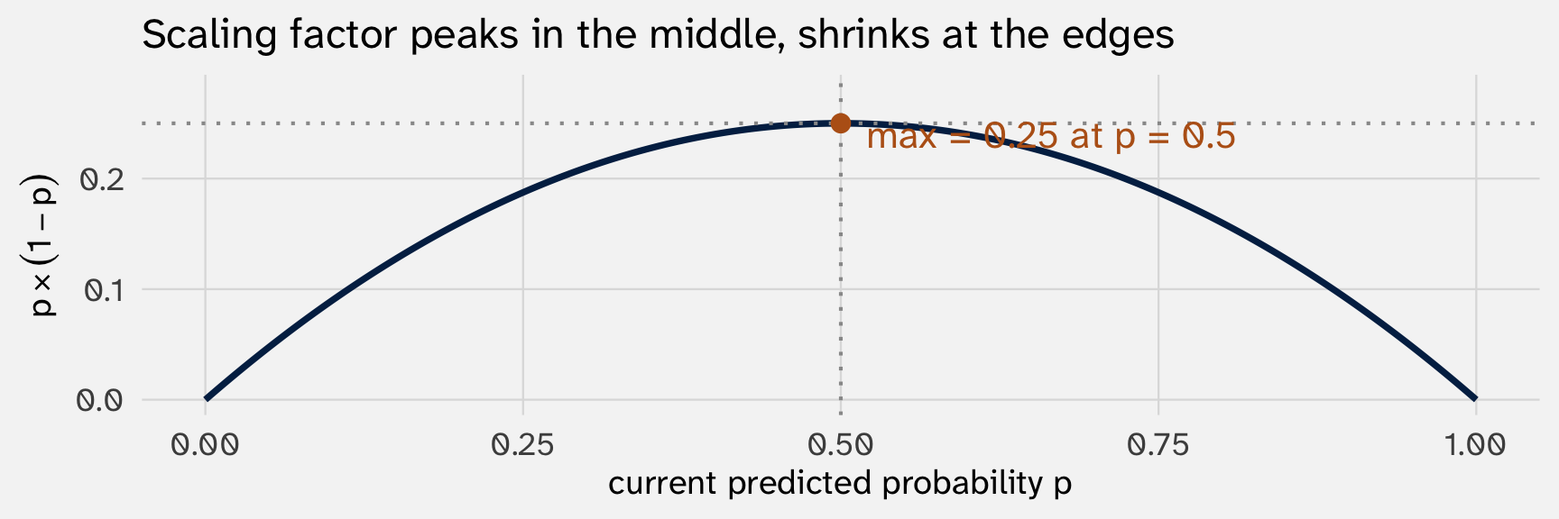
| baseline \(p\) | scaling \(p(1-p)\) | ME for \(\beta = 1\) |
|---|---|---|
| 0.1 | 0.09 | 0.09 |
| 0.5 | 0.25 | 0.25 |
| 0.9 | 0.09 | 0.09 |
→ Same \(\beta\), different probability-effects at different baselines. This is why logit effects require a scenario to interpret
With controls: it depends on \(X\) and the controls
Now add controls. The linear predictor becomes:
\[z \;=\; \beta_0 + \beta_1 X + \beta_2 Z_1 + \beta_3 Z_2 + \cdots\]
The marginal-effect formula is the same:
\[\frac{dP}{dX} \;=\; \sigma(z)\,(1 - \sigma(z)) \cdot \beta_1\]
But now \(z\) depends on the values of all the controls. So the effect of \(X\) depends on:
- The value of \(X\) itself (where on the sigmoid you are because of \(X\))
- The values of every other covariate (where on the sigmoid you are because of the rest of your profile)
The ME of being Protestant depends on age
Concrete: for wall ~ protestant + age, the marginal effect of being Protestant on Pr(wall) depends on the respondent’s age.
# logit of wall support on Protestant + age
mod_wall = glm(wall ~ protestant + age, data = bot_clean, family = binomial())

# contrast: Pr(wall | Protestant) - Pr(wall | Non-Protestant), across age
me_prot = comparisons(mod_wall, variables = "protestant",
                      newdata = datagrid(age = seq(20, 85, by = 5)))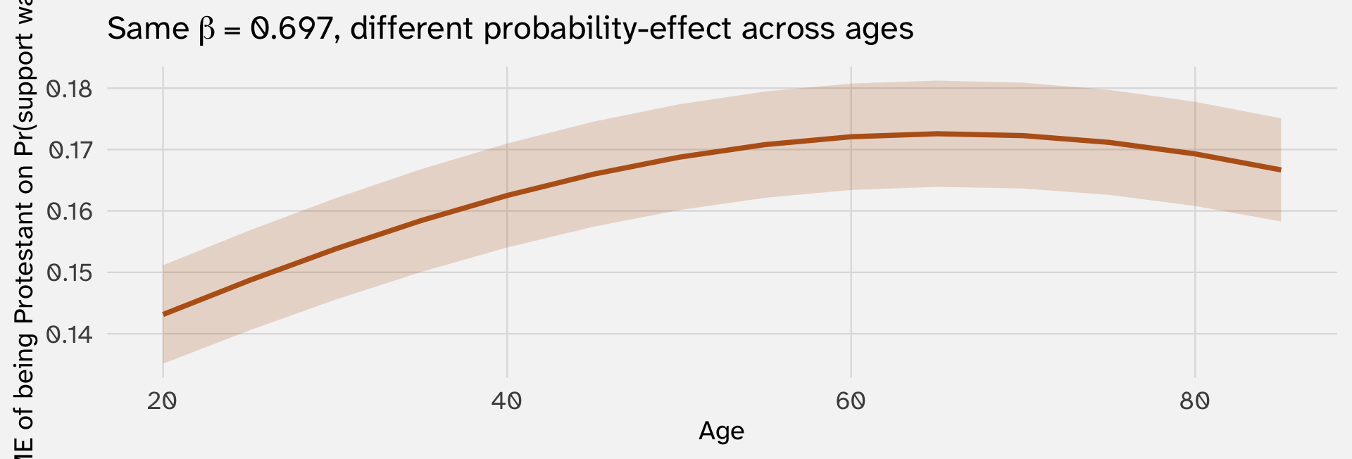
To interpret \(\beta_1\), set a scenario and predict
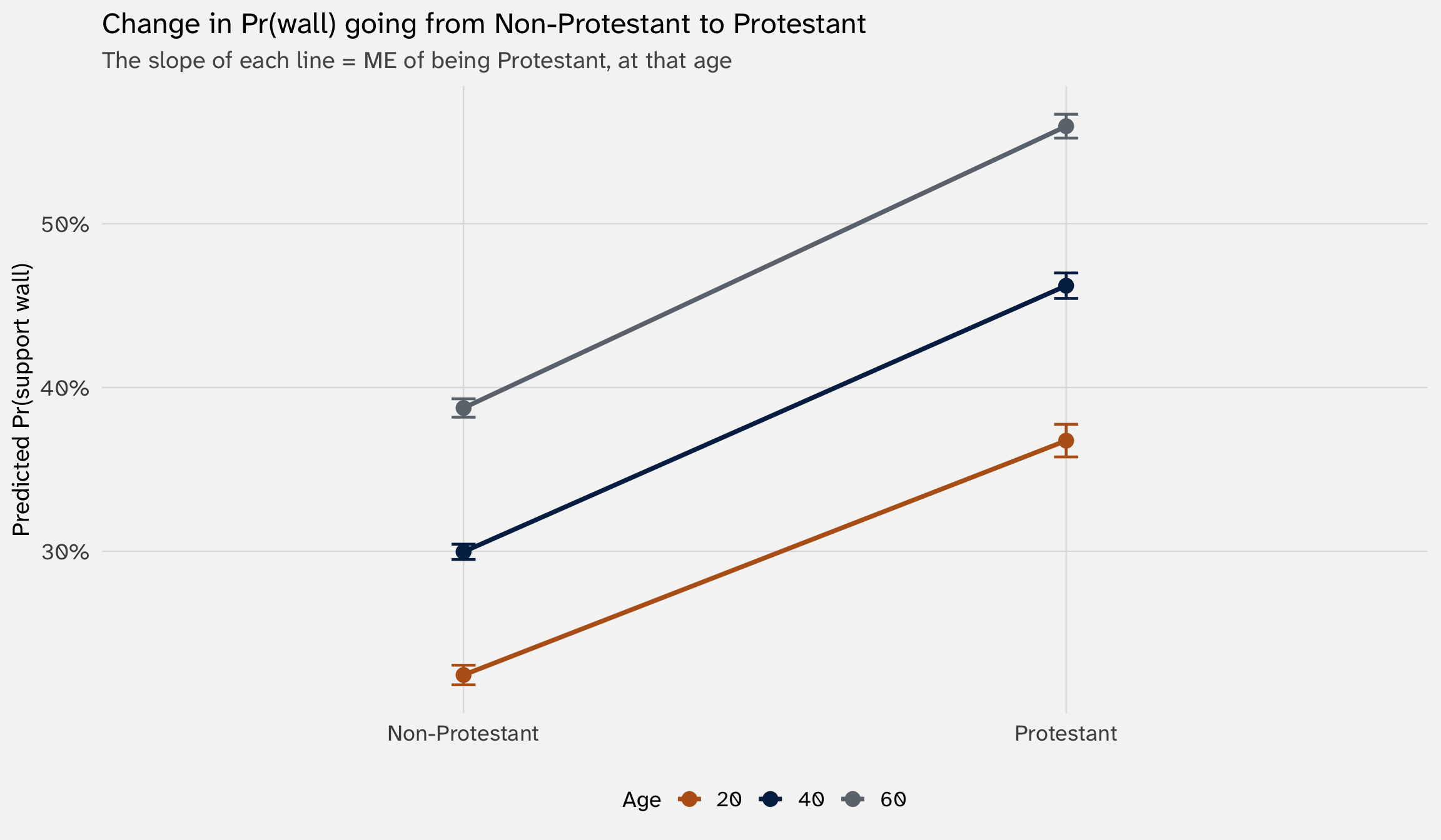
The Average marginal effect
The marginaleffects::comparisons/slopes() estimates marginal effects for every row in your data:
 Estimate Std. Error    z Pr(>|z|)   S 2.5 % 97.5 %
    0.170    0.00442 38.6   <0.001 Inf 0.162  0.179
    0.173    0.00442 39.1   <0.001 Inf 0.164  0.181
    0.171    0.00437 39.2   <0.001 Inf 0.163  0.180
    0.172    0.00442 38.8   <0.001 Inf 0.163  0.180
    0.170    0.00441 38.6   <0.001 Inf 0.161  0.179
    0.172    0.00442 38.9   <0.001 Inf 0.163  0.181

Term: protestant
Type: response
Comparison: Protestant - Non-Protestant
marginaleffects::avg_comparisons/avg_slopes() averages over all these individual effects
When does LPM = logit?
Fit both models on wall ~ protestant (no controls), compare predicted probabilities:
mod_lpm   = lm(wall  ~ protestant, data = bot_clean)
mod_logit = glm(wall ~ protestant, data = bot_clean, family = binomial())

scenarios_simple = tibble(protestant = c("Non-Protestant", "Protestant")) |>
  mutate(LPM   = predict(mod_lpm,   newdata = pick(everything())),
Logit = predict(mod_logit, newdata = pick(everything()), type = "response"))| protestant | LPM | Logit |
|---|---|---|
| Non-Protestant | 0.330 | 0.330 |
| Protestant | 0.524 | 0.524 |
Identical → with one binary predictor and no controls, both models just compute group means
When does LMP not equal logit?
Now add age as a control:
mod_lpm2   = lm(wall  ~ protestant + age, data = bot_clean)
mod_logit2 = glm(wall ~ protestant + age, data = bot_clean, family = binomial())

scenarios_ctrl = crossing(protestant = c("Non-Protestant","Protestant"), age = c(20, 50, 80)) |>
  mutate(LPM   = predict(mod_lpm2,   newdata = pick(everything())),
         Logit = predict(mod_logit2, newdata = pick(everything()), type = "response"),
diff = Logit - LPM)| protestant | age | LPM | Logit | diff |
|---|---|---|---|---|
| Non-Protestant | 20 | 0.213 | 0.224 | 0.011 |
| Non-Protestant | 50 | 0.347 | 0.342 | -0.005 |
| Non-Protestant | 80 | 0.480 | 0.483 | 0.003 |
| Protestant | 20 | 0.378 | 0.368 | -0.011 |
| Protestant | 50 | 0.512 | 0.511 | -0.001 |
| Protestant | 80 | 0.645 | 0.653 | 0.007 |
Close, not identical → divergence grows at the extremes of the covariate range, where the sigmoid bends and the LPM straight line cannot
→ LPM = logit when: there are no continuous covariates and no nonlinearities in \(X\beta\). With binary X only, both models just recover the cell means
Logit vs. LPM visualized
Same data, two models, one picture:
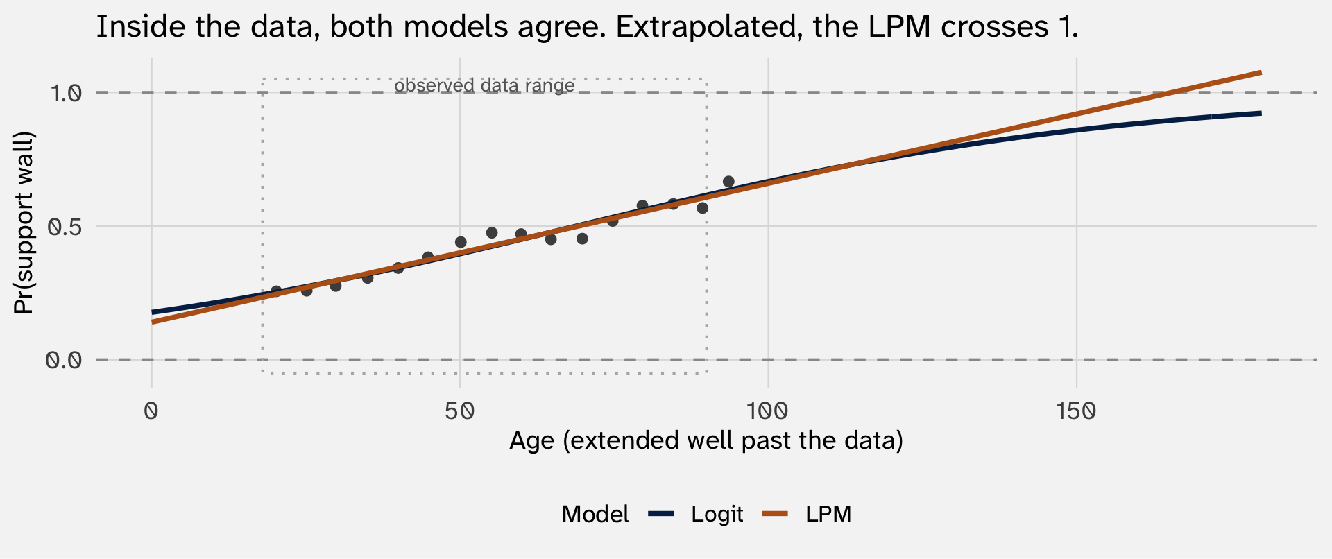
Within the data: LPM and logit make essentially the same predictions. Extrapolated: the LPM line reaches Pr = 1 at age 165, then keeps going
📝 Activity: interpret a logit
Back to the affairs dataset (Fair 1978, n = 601)
- Fit a logit of having an affair against having kids and how long the person has been married
- Interpret the coefficient on
years_marriedthree ways:- as a log-odds coefficient, (b) as an odds ratio (
exp(β))
- as a log-odds coefficient, (b) as an odds ratio (
- Plot predicted \(\Pr(\text{affair})\) across
years_married, separately for people with and without kids - Plot the Marginal Effect of
years_marriedacross years married, separately for people with and without kids - Calculate the AME to the LPM coefficient — are they similar?
What should I report?
So many results; here’s what you should put in a paper:
The raw coefficients
tidy(mod_logit) output as a regression table → not interpretable, but useful to catch potential problems → Appendix
Average marginal effect
avg_comparisons() → one probability-scale number. Nice top-level result
Predicted probability plot
augment()/predictions + ggplot → shows how Pr\((Y=1)\) varies across \(X\), holding controls fixed
Common pitfalls with logit
1. Don’t read \(\beta\) as a probability change. It is in log-odds units. Always convert (AME, scenario, or odds ratio)
2. There is no single “effect.” The marginal effect depends on the full covariate profile — always state the scenario or report the AME
3. Coefficients shift with the model. Adding or removing covariates changes every coefficient, even the intercept, because the link is nonlinear. Coefficients are not “partial effects” in the OLS sense
4. Perfect separation breaks the model. If some covariate perfectly predicts \(Y\), glm() returns huge coefficients and warnings about “fitted probabilities numerically 0 or 1” → you’ll know when you see \(|\hat\beta| > 10\) with massive SEs. We’ll discuss next week