| country | leader | duration | event | age_start | mil_service | combat | rebel |
|---|---|---|---|---|---|---|---|
| AFG | Amin | 1 | 1 | 50 | 1 | 1 | 1 |
| AFG | Habibullah Ghazi | 1 | 1 | 39 | 1 | 0 | 1 |
| AFG | Hamid Karzai | 14 | 1 | 44 | 0 | 0 | 0 |
| ALG | Bouteflika | 17 | 0 | 62 | 0 | 0 | 1 |
| ANG | Dos Santos | 37 | 0 | 37 | 0 | 0 | 1 |
| BAH | Hamad Isa Ibn Al-Khalifah | 17 | 0 | 49 | 1 | 0 | 0 |
Duration Models
POL 213 · Week 6
Juan F. Tellez
University of California, Davis
May 6, 2026
Housekeeping
- Midterm grades returned
- PS5 released today; covers count models + duration
Where we are
Six weeks so far
Wk 1: OLS
\[Y = X\beta + \varepsilon\]
Continuous \(Y\)
Wk 2: Transformed
\[Y = f(X)\beta + \varepsilon\]
You chose nonlinearity
Wk 3: Logit
\[\Pr(Y=1) = \sigma(X\beta)\]
Binary \(Y\)
Wk 4: MLE
glm(...) — maximize the likelihood
Wk 5: Counts
\[Y \in \{0, 1, 2, \ldots\}\]
Poisson, NB
Wk 6: Duration
\[Y = \text{time to event}\]
A fourth outcome type
Today: same MLE engine, new outcome type, one structurally new ingredient → censoring
1. Time-to-event in political science
Time-to-event outcomes are everywhere
Some research questions are about how long until something happens:
- Why are some leaders in power many years, others for briefer periods? (time until leader leaves office)
- Why do some civil wars last longer than others? (time until a civil war ends)
- Why do some peace agreements last for years, others collapse quickly? (time until peace agreement fails)
- Why did some countries democratize more quickly than others? (time until a country becomes a democracy)
- Why do some cabinets last longer than others? (time until a cabinet is voted out)
These outcomes share a structure:
- a non-negative random variable \(T \geq 0\) (a unit’s duration / time-to-event),
- often right-skewed,
- and — critically — some observations are not yet over when the data ends
Today’s data: leader survival in office (1840–2015)
Each row = one leader’s complete spell in office in a country. Records the leader’s time in office and characteristics at the start of the spell.
Important = when the data was collected (2015), some leaders were still in office (had not completed their spell)
event = 1→ leader left office during 1840–2015 (the spell is complete)event = 0→ leader was still in office in 2015 (the spell is right-censored)
Censoring is common in duration data
Right-censored spells are observations we couldn’t follow to the end. We know the leader lasted at least duration years — but their true survival time is unknown to us
| country | leader | duration | end_year | age_start | edu | mil_service | combat | rebel | event |
|---|---|---|---|---|---|---|---|---|---|
| AFG | Taraki | 2 | 1979 | 61 | Secondary | 0 | 0 | 1 | 1 |
| SOL | Sogavare | 2 | 2015 | 46 | University | 0 | 0 | 0 | 0 |
Problem: Taraki and Sogavare are observationally equivalent — they appear to have survived the same amount of time, when they haven’t
Censoring is the structurally novel feature of duration data; one reason OLS doesn’t quite work
Does a rebel background extend leader survival?
Goal: estimate the effect of a rebel background (rebel) on leader survival (duration, event), controlling for age, education, military service, prior combat experience
Substantive question: do leaders who came to power through armed rebellion last longer in office (consolidated networks of loyalty forged in the rebellion, hard-won coercive infrastructure) or shorter (volatile post-conflict regimes, ongoing contests over legitimacy)?
What does rebel = 1 mean?
Indicator for whether the leader personally participated in an armed rebellion before coming to power — guerrilla movements, insurgencies, wars of national liberation. About 26% of leader-spells in the data have it.
What does the outcome look like?
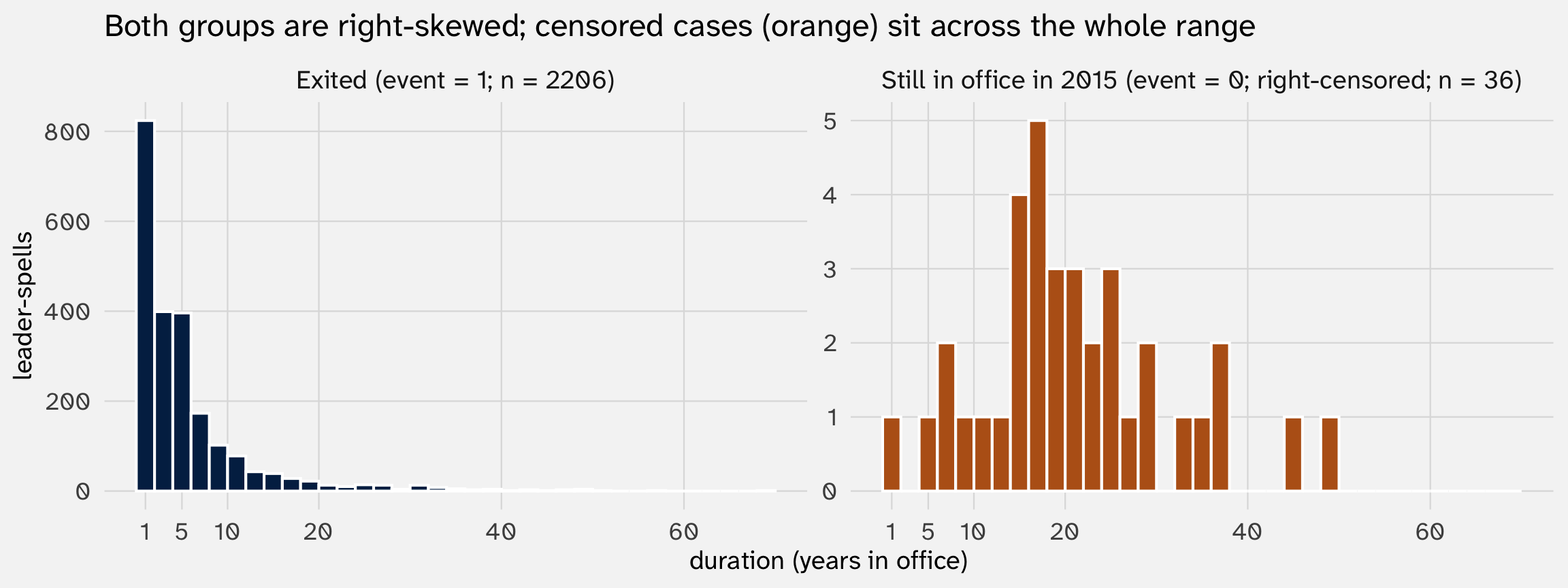
Key features:
- Non-negative, often integer-valued: \(T \geq 0\)
- Long right tail: most leaders last < 10 years; a few last 30+
- Right-censoring: ~2% of spells are unfinished at the end of the sample
Could we just use OLS?
| OLS on duration | |
|---|---|
| + p < 0.1, * p < 0.05, ** p < 0.01, *** p < 0.001 | |
| Intercept | 17.542*** |
| (0.724) | |
| age_start | -0.227*** |
| (0.013) | |
| mil_service | 0.731 |
| (0.531) | |
| combat | -0.341 |
| (0.584) | |
| rebel | 1.009** |
| (0.375) | |
| Num.Obs. | 2242 |
| R2 | 0.127 |
2. Why not OLS on a duration outcome?
Three problems
1. OLS predicts negative durations — but \(T \geq 0\) by definition. Same support problem as Poisson on counts
2. Durations are typically log-skewed — variance grows with the mean. OLS standard errors are wrong
3. OLS has no way to handle censoring — and every option for dealing with it is biased
- and (2) are familiar problems. (3) is the structural problem that motivates duration models
Problem 3: censoring breaks every OLS shortcut
duration mixes up two things:
- leaders whose spell lasted \(X\) years in office, and
- leaders who by the time the data was collected had spent \(X\) years in office
What can we do?
Option A — pretend censored spells ended at their last observation (i.e., set duration = end_year - start_year, treat as completed). Bad. You’re treating “still in office at 2015” as “exited in 2015” → systematically under-counts long survivors
Option B — drop censored observations (filter to event == 1, then OLS). Bad. This is the opposite selection: you keep only the leaders we got to see exit, throwing away the long-lasting incumbents — over-counts short survivors
A simulation: censoring really does bias OLS
We can’t show bias on the leaders data — we don’t know each leader’s true survival time, only what we observed before 2015
Simulation — if we generate the data ourselves, we know each leader’s true spell length even when we then “censor” it at \(C\). We can compare what OLS would have estimated with full information against what it estimates with censoring → the bias is the difference
The DGP — same variable names as the leaders data; just one predictor (rebel), no controls:
set.seed(213)
n        = 2000
rebel    = rbinom(n, size = 1, prob = 0.5)                # binary "rebel background"
dur_true = rexp(n, rate = ifelse(rebel == 1, 0.1, 0.2))   # rebel=1 → mean 10; rebel=0 → mean 5
C        = 7                                              # censoring threshold (years of follow-up)
event    = as.integer(dur_true <= C)                      # exited before C?
duration = pmin(dur_true, C)                              # what we actually see
sim      = tibble(rebel, dur_true, duration, event)
True effect of rebel on \(\mathbb{E}[\text{duration}]\) = \(10 - 5 = 5\) (years of extra tenure)
Three views of the same simulated data
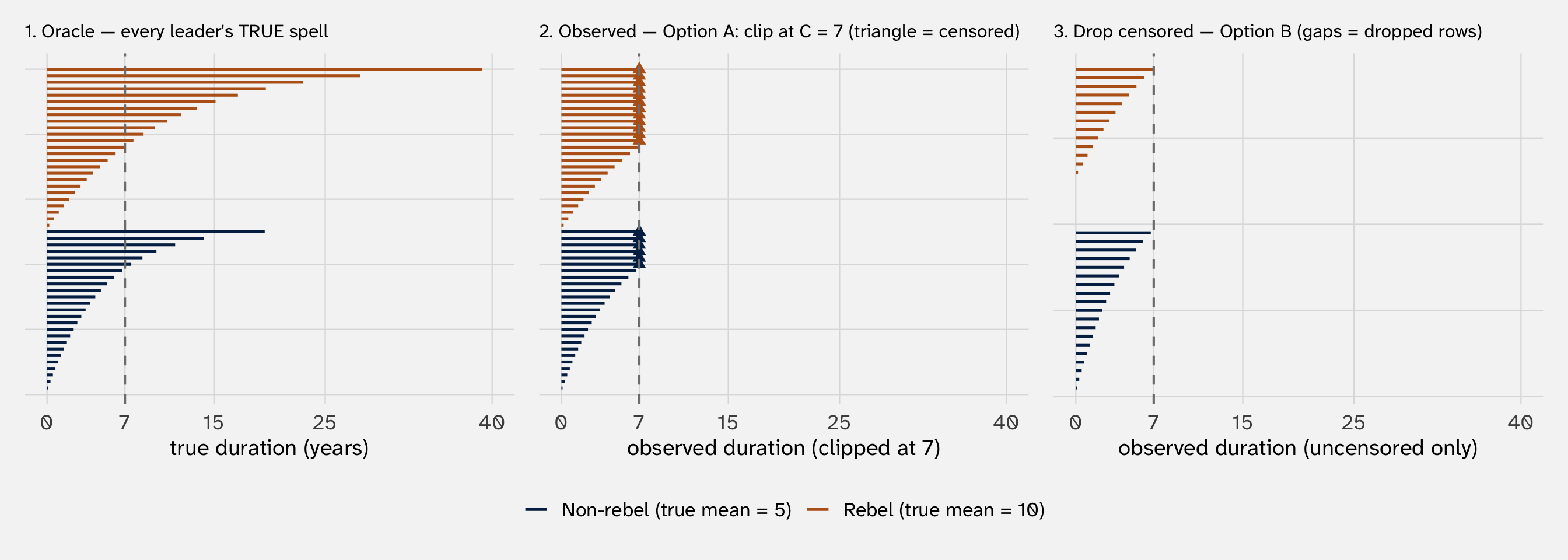
What should these do to our treatment (rebel, yes/no) effect?
- Option A clips long survivors at 7 (the right edge of the bars gets cut off) → estimated rebel effect shrinks
- Option B drops the long survivors entirely (the gaps in panel 3 are mostly orange) → estimated rebel effect shrinks even more
Both approaches fail
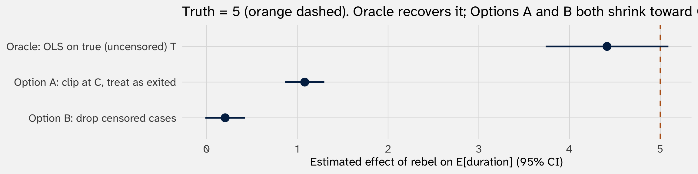
The oracle nails it → OLS isn’t broken; censoring is what breaks OLS. Both shortcuts shrink the estimate toward 0 because censoring clips long survivors, and the clipping hits the rebel = 1 (long-living) group harder
What we actually need
A model that:
- Respects the support \(T \geq 0\) — like Poisson does for counts
- Acknowledges the skew — like log-transforms in Week 2
- Uses censored observations correctly — new ingredient: censored cases contribute “we know \(T > t_i\)” rather than “\(T = t_i\)”
That’s exactly what duration models do. The first two are familiar from count week. The third is what makes this week different
3. The survival function and Kaplan-Meier
A subtle shift in the question
We can’t always answer “how long does a leader last in office?” for any given leader because of censoring
But we can answer “what fraction of leaders are still in office after \(t\) years?” — this is computable at any \(t\), even with censored cases sitting in the data
This is the survivor function:
\[S(t) = \Pr(T > t)\]
where \(T\) is a leader’s duration in office (random variable); \(t\) is a specific number of years we plug in
Two equivalent readings of the same number:
- Probability (one leader): an arbitrary leader’s chance of staying in office past \(t\)
- Fraction (all leaders): the share of all leaders who stay in office past \(t\)
e.g., \(S(5) = 34\%\) → 34% of leaders are still in office at year 5; the other 66% (= \(1 - S(5)\)) have already exited
What does \(S(t)\) look like for our leaders?
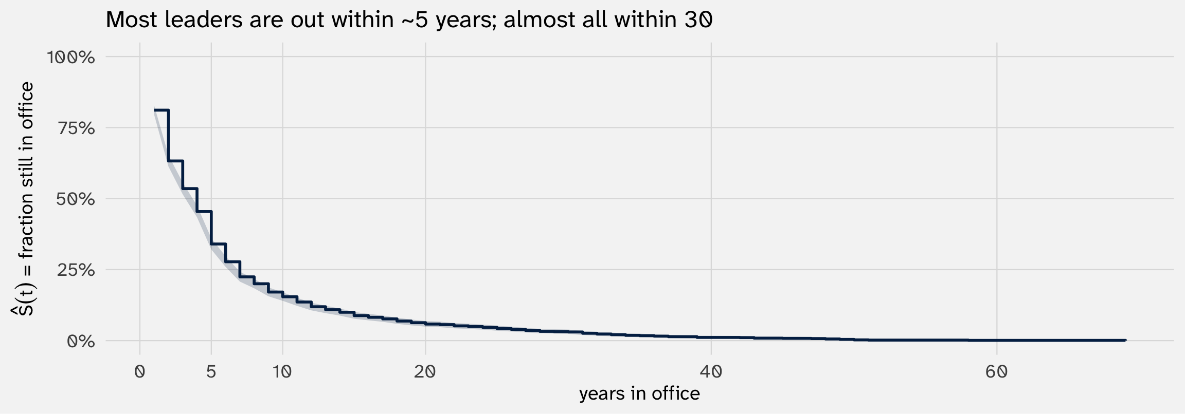
Read it directly: at \(t = 5\), ~34% of leaders are still in office. We just need a way to compute this curve that handles censored cases correctly → that’s Kaplan-Meier
Surv(duration, event) pairs the time variable with the censoring variable
The ~ 1 means “no covariates, just the overall curve”
Kaplan-Meier: how censored cases are used
In §2 we said we needed a way to use “this leader survived at least \(t_i\) years” — without dropping the spell or pretending it ended. KM does exactly this.
The trick: at each moment when an exit happens, KM asks “of those still at risk right now, what fraction failed?” Censored cases sit in the denominator until they’re censored, then leave without contributing an event
Worked example: 5 leaders
The data
| leader | dur | event |
|---|---|---|
| A | 2 | 1 (exit) |
| B | 3 | 0 (cens) |
| C | 5 | 1 (exit) |
| D | 7 | 1 (exit) |
| E | 8 | 0 (cens) |
Stepping through events to build \(\hat S(t)\)
| \(t\) | at risk | what happens | \(\hat S(t)\) |
|---|---|---|---|
| 0 | 5 | — | \(1.00\) |
| 2 | 5 | A exits | \(1.00 \times (1 - \tfrac{1}{5}) = 0.80\) |
| 3 | 4 | B censored | stays at \(0.80\) |
| 5 | 3 | C exits | \(0.80 \times (1 - \tfrac{1}{3}) = 0.53\) |
| 7 | 2 | D exits | \(0.53 \times (1 - \tfrac{1}{2}) = 0.27\) |
| 8 | 1 | E censored | stays at \(0.27\) |
B and E are not thrown away — they sit in the denominator at every event time before they’re censored, contributing “we know they made it this far.” When censored, they leave without an event. That’s how KM accounts for censored observations.
KM by group: rebel background vs. not
KM lets us see the gap: rebel leaders stick around longer
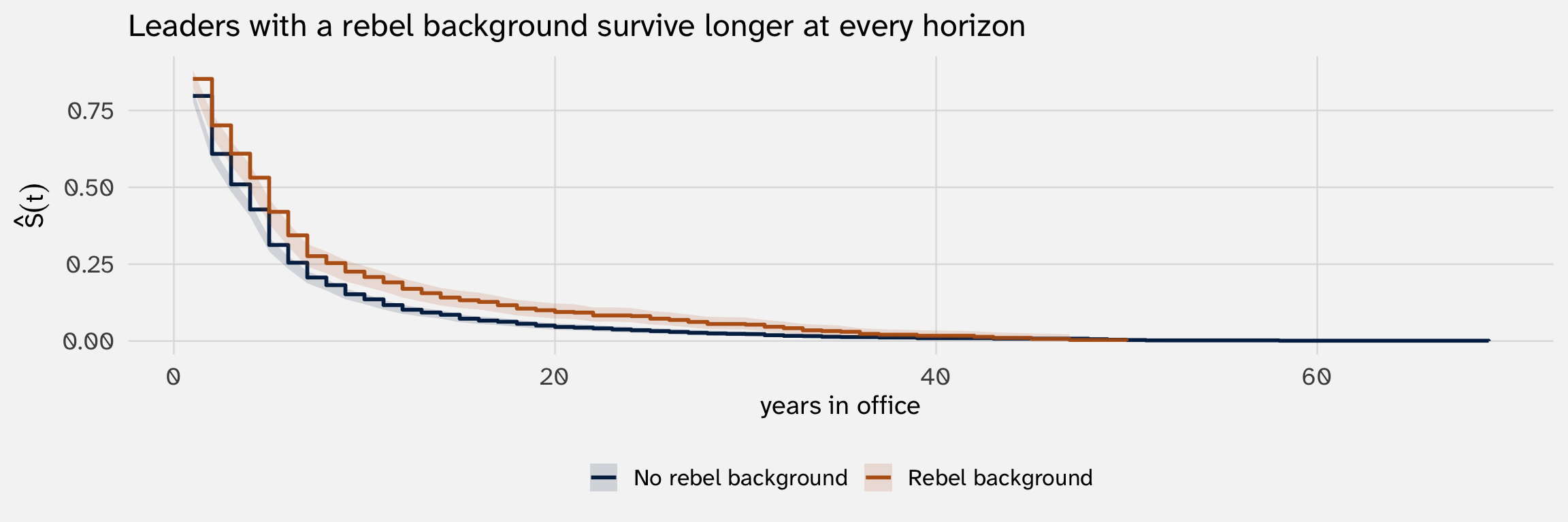
But this is descriptive — no covariates beyond the grouping variable. To control for age, education, etc., we need a regression model
4. Parametric duration models — exponential MLE
Three models of increasing complexity: exponential, Weibull, and Cox proportional hazard
From KM to regression
KM gave us \(\hat S(t)\) → nice, but limited as a tool for inference
What KM can’t do:
- Multiple covariates at once — stratifying KM by
rebelwas easy; byrebel × age × edu × …splits the sample into useless slivers - Hold covariates constant — there’s no “effect of
rebelholdingagefixed” in a KM curve - Predicted survival at a chosen scenario — KM gives one curve, not a family of curves indexed by \(X\)
The fix: write \(S(t)\) as a parametric function of \(X\) and \(\beta\), then estimate \(\beta\) via MLE — same Week 4–5 machinery, on a likelihood that handles censoring (censored cases will contribute their \(S(t_i)\), exactly as they sat in KM’s at-risk denominator)
The simplest such model → exponential. One parameter; a constant hazard
The exponential: a simple duration model
We said the goal is to parameterize \(S(t)\). In practice, we parameterize the hazard rate \(h(t)\) — and \(S(t)\) falls out automatically, because the two are linked by a formula:
\[S(t) = \exp\!\Big(- \!\int_0^{\,t} h(u)\, du\Big)\]
→ pick a form for \(h(t)\), and \(S(t)\) is fully determined. (Concretely: if \(h(t) = \lambda\), then \(S(t) = e^{-\lambda t}\).)
Why is \(h\) the easier place to put \(X\beta\)? \(h\) is a positive rate with no upper bound — perfect for a log link: \(\log h = X\beta\), exactly like Poisson’s log-rate. Putting \(X\beta\) directly on \(S \in [0, 1]\) would need a more awkward link to keep predictions in-bounds
What is a hazard rate?
The hazard rate — the rate of failure for those who’ve made it to time \(t\):
\[h(t) = \lambda(t) = \text{rate of failure at time } t \text{ given } T \geq t\]
For our leader data: The empirical rate is just
\[\hat\lambda \;=\; \frac{\text{observed exits } (\text{event} = 1)}{\text{person-years at risk}} \;=\; \frac{2206}{13918} \;\approx\; 0.16 \text{ per year}\]
Reading: about 16% of leaders still in office exit per year — equivalent to a mean tenure of \(1/\hat\lambda \approx\) 6.3 years
Add covariates via the log link:
\[\log \lambda_i = X_i \beta \qquad\Longleftrightarrow\qquad \lambda_i = e^{X_i \beta}\]
Now each leader has their own \(\lambda_i\), set by their covariates: constant over time within a leader, varying across leaders with \(X\). Same log-rate scale as Poisson — same machinery transfers
The likelihood with censoring
Let \(\delta_i\) = event indicator:
\[\mathcal{L}(\beta) = \prod_{i=1}^n \bigl[f(t_i)\bigr]^{\delta_i} \bigl[S(t_i)\bigr]^{1 - \delta_i}\]
Uncensored observations (we saw the leader exit at \(t_i\)) contribute the density of exit times \(f(t_i)\) — Higher \(f(t_i)\) means our model says “yes, an exit at that time is plausible.”
\[f(t_i; \lambda_i) = \underbrace{\lambda_i}_{\substack{\text{rate of exit} \\ \text{(hazard)}}} \cdot \underbrace{e^{-\lambda_i t_i}}_{\substack{\text{probability of} \\ \text{surviving to } t_i}}\]
Censored observations (we know \(T > t_i\) — the leader was still in office) contribute the survivor function \(S(t_i)\) — the probability of having lasted at least \(t_i\) years:
\[S(t_i; \lambda_i) = e^{-\lambda_i t_i}\]
We want \(\beta\) to make exited spells plausibly timed and censored spells plausibly long-lasting
Concrete: what does “plausibly timed” actually mean?
Two leaders, two candidate values of \(\lambda\). Each leader contributes its log-likelihood term to a running sum:
| exit observed (event = 1) | censored (event = 0) | |
|---|---|---|
| Likelihood term | \(f(t_i; \lambda) = \lambda \, e^{-\lambda t_i}\) | \(S(t_i; \lambda) = e^{-\lambda t_i}\) |
| Log-likelihood term | \(\log \lambda - \lambda t_i\) | \(-\lambda t_i\) |
Leader A exits at \(t_A = 2\). Leader B is censored at \(t_B = 10\).
Model 1: \(\lambda = 0.5\)
(high rate, mean tenure \(1/\lambda = 2\) yrs)
- Leader A: \(\log(0.5) - (0.5)(2)\) \(= -0.69 - 1.00 = -1.69\)
- Leader B: \(-(0.5)(10) = -5.00\)
- Total: \(-1.69 + (-5.00) = -6.69\)
Model 2: \(\lambda = 0.1\)
(low rate, mean tenure \(1/\lambda = 10\) yrs)
- Leader A: \(\log(0.1) - (0.1)(2)\) \(= -2.30 - 0.20 = -2.50\)
- Leader B: \(-(0.1)(10) = -1.00\)
- Total: \(-2.50 + (-1.00) = \mathbf{-3.50}\) ← higher
Model 2 wins: it balances both observations. Model 1’s high hazard makes B’s long tenure implausibly unusual (\(-5\) penalty); Model 2’s low hazard makes A’s quick exit only slightly early (\(-2.5\)). MLE picks the \(\lambda\) that maximizes the sum — the analog of OLS minimizing \(\sum(y_i - \hat y_i)^2\)
Fit an exponential model in R
| Exponential | |
|---|---|
| + p < 0.1, * p < 0.05, ** p < 0.01, *** p < 0.001 | |
| (Intercept) | 3.252*** |
| (0.097) | |
| age_start | -0.030*** |
| (0.002) | |
| mil_service | 0.071 |
| (0.077) | |
| combat | -0.016 |
| (0.086) | |
| rebel | 0.238*** |
| (0.053) | |
| Num.Obs. | 2242 |
Coefficients are on the log of expected survival time scale — called the accelerated failure time (AFT) parameterization, because covariates stretch or compress event times
Positive coefficient → longer survival; negative → shorter. Same multiplicative structure as Poisson rate coefficients — just on the time scale instead of the count scale → next slide
Interpretation 1: exponentiate \(\hat\beta\) → time ratio
# A tibble: 4 × 5
  term        time_ratio conf.low conf.high  p.value
  <chr>            <dbl>    <dbl>     <dbl>    <dbl>
1 age_start        0.970    0.967     0.974 3.74e-65
2 mil_service      1.07     0.923     1.25  3.55e- 1
3 combat           0.984    0.832     1.16  8.50e- 1
4 rebel            1.27     1.14      1.41  6.70e- 6
Read it: \(\exp(\hat\beta_{\text{rebel}}) \approx\) 1.27 → rebel-background leaders survive about 27% longer than non-rebels in expectation, holding other covariates fixed
Same multiplicative interpretation we saw with Poisson rate ratios → just on the time scale
Way 2: predicted survival at chosen scenarios
# A tibble: 2 × 4
  rebel estimate conf.low conf.high
  <dbl>    <dbl>    <dbl>     <dbl>
1     0     5.39     5.10      5.67
2     1     6.83     6.14      7.53
Read it: a typical leader has predicted expected survival of ~X years without a rebel background, vs. ~Y years with one. The difference in predicted survival is the substantive ATE-like quantity readers want
Way 2 (visual): same scenarios as full survival curves
Exponential has a closed-form \(\hat S(t \mid X) = \exp(-t / \exp(X\hat\beta))\), we can plot using flexsurv:
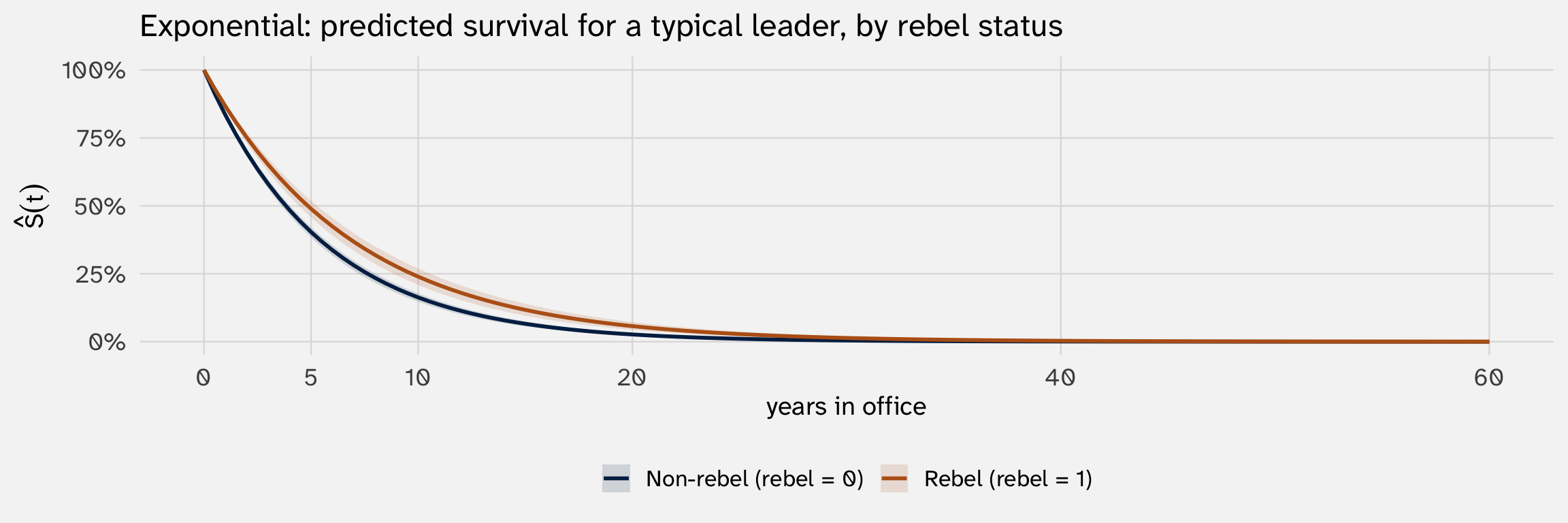
The two predicted means we just computed are the areas under these two curves — the rebel curve sitting above the non-rebel curve at every \(t\) is what gives rebels longer expected tenure
Why flexsurv for the plot?
survreg doesn’t return CIs for \(\hat S(t \mid X)\) out of the box. flexsurv::flexsurvreg() is a drop-in replacement (same MLE, same coefficients, just a different package interface) whose summary() method returns predicted survival with confidence intervals already computed at any newdata × t grid
Way 3: marginal effect of \(X\) on \(\mathbb{E}[T]\)
You’d get to it via calculus, but we can just state the result:
\[\frac{\partial \, \mathbb{E}[T \mid X]}{\partial X_k} = \hat\beta_k \cdot \mathbb{E}[T \mid X]\]
The effect of \(X\) on \(\mathbb{E}[T]\) scales with \(\mathbb{E}[T]\) itself — exactly like Poisson, where the effect on the count scaled with the count. Long-lived leaders feel a 1-unit change in \(X\) as more years of difference; short-lived leaders feel less
5. Constant hazard is too rigid — Weibull
The exponential’s hidden assumption
Exponential says: \(h(t) = \lambda\) — the hazard is the same at every \(t\)
For leaders, that says: a leader’s risk of being ousted is the same in year 1 as in year 30. Plausible?
The data (and theory!) say no: hazards usually change with time. Honeymoons, consolidation, term limits, exhaustion
Weibull: let the hazard rise or fall with \(t\)
The Weibull model adds a shape parameter \(p\):
\[h(t) = \lambda \, p \, (\lambda t)^{p - 1}\]
- \(p = 1\) → exponential (constant hazard) — the special case
- \(p > 1\) → hazard rises with \(t\) (positive duration dependence)
- \(p < 1\) → hazard falls with \(t\) (negative duration dependence)
Same nesting story as Poisson ⊂ NB — exponential is a special case of Weibull. Fit Weibull, check if \(\hat p \approx 1\); if so, exponential is fine
Fit a Weibull in R
| Exponential | Weibull | |
|---|---|---|
| + p < 0.1, * p < 0.05, ** p < 0.01, *** p < 0.001 | ||
| (Intercept) | 3.252*** | 3.303*** |
| (0.097) | (0.087) | |
| age_start | -0.030*** | -0.030*** |
| (0.002) | (0.002) | |
| mil_service | 0.071 | 0.068 |
| (0.077) | (0.069) | |
| combat | -0.016 | -0.011 |
| (0.086) | (0.076) | |
| rebel | 0.238*** | 0.241*** |
| (0.053) | (0.047) | |
| Log(scale) | -0.113*** | |
| (0.016) | ||
| Num.Obs. | 2242 | 2242 |
Coefficients usually move a bit. The shape parameter \(\hat p\) doesn’t appear in the regression table — survreg stores it separately. We extract it next
Was constant hazard OK?
survreg parameterizes Weibull as \(\log T = X\beta + \sigma W\). The Log(scale) row in the regression table is the MLE of \(\log \hat\sigma\) — and the Weibull shape is \(\hat p = 1/\hat\sigma\):
How to read \(\hat p\):
- \(\hat p \approx 1\) → exponential (constant hazard) is fine
- \(\hat p > 1\) → hazard rises with \(t\) (leaders’ exit risk grows the longer they’re in office)
- \(\hat p < 1\) → hazard falls with \(t\) (if you survive the early years, you’re safer)
For our data: \(\hat p \approx\) 1.12 → some duration dependence; constant hazard is approximately, but not perfectly, OK
Interpretation: same three-step workflow, condensed
Coefficients on the log-time scale. The whole exponential interpretation arc transfers verbatim:
Way 1 — exponentiate \(\hat\beta\) → time ratio
# A tibble: 4 × 5
  term        time_ratio conf.low conf.high  p.value
  <chr>            <dbl>    <dbl>     <dbl>    <dbl>
1 age_start        0.970    0.967     0.973 2.45e-83
2 mil_service      1.07     0.935     1.23  3.25e- 1
3 combat           0.989    0.851     1.15  8.85e- 1
4 rebel            1.27     1.16      1.40  3.06e- 7
Way 2 — predicted survival at chosen scenarios: same predictions(mod_wb, newdata = datagrid(rebel = c(0, 1))) as exponential
Way 3 — formula for ME on \(\mathbb{E}[T]\): same multiplicative structure as exponential — \(\partial \mathbb{E}[T]/\partial X_k = \hat\beta_k \cdot \mathbb{E}[T \mid X]\). AME via avg_slopes(mod_wb, variables = "rebel")
The substantive headline is preserved — rebel-background leaders survive about 27% longer in expectation
Way 2 (visual): Weibull predicted survival curves
Weibull has a closed-form \(\hat S(t \mid X) = \exp\!\bigl(-(t/\exp(X\hat\beta))^{\hat p}\bigr)\) — same plot recipe as the exponential, with flexsurv again giving us CIs:
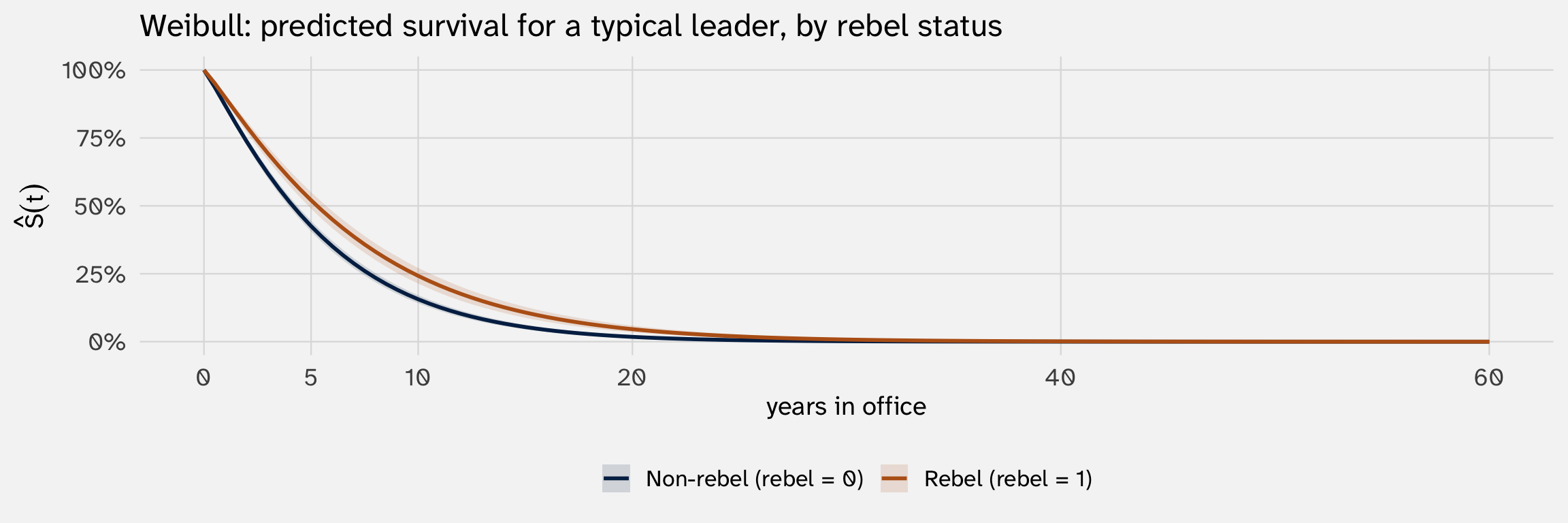
Same vertical-gap reading as exponential — but the curves now have a slight bend reflecting non-constant hazard (\(\hat p \neq 1\))
6. Cox proportional hazards
What if I don’t want to commit to a hazard shape?
Every duration model has a baseline hazard \(h_0(t)\) — the hazard curve for a “reference” leader (all \(X = 0\)): how does their exit risk evolve over time? Exp and Weibull force this curve into a fixed shape:
| Model | \(h_0(t)\) formula | Shapes it can represent |
|---|---|---|
| Exponential | \(\lambda\) | Only flat (constant) |
| Weibull | \(\lambda p (\lambda t)^{p-1}\) | Only monotone (rising or falling, but not both) |
If the true baseline hazard rises, plateaus, then falls (early instability → consolidation → late-stage challenges), neither model can capture it — they’ll smooth it into a single line
Cox’s move: don’t pick a formula for \(h_0(t)\) at all. Let it be whatever the data suggests — flat, monotone, U-shaped, lumpy, anything — and just model how covariates scale that whole curve up or down:
\[h(t \mid X) = \underbrace{h_0(t)}_{\text{shape: free}} \;\cdot\; \underbrace{\exp(X\beta)}_{\substack{\text{level shift:}\\ \text{constant in }t}}\]
Fit a Cox model — side by side with Exp & Weibull
| Exponential | Weibull | Cox PH | |
|---|---|---|---|
| + p < 0.1, * p < 0.05, ** p < 0.01, *** p < 0.001 | |||
| (Intercept) | 3.252*** | 3.303*** | |
| (0.097) | (0.087) | ||
| age_start | -0.030*** | -0.030*** | 0.029*** |
| (0.002) | (0.002) | (0.002) | |
| mil_service | 0.071 | 0.068 | -0.066 |
| (0.077) | (0.069) | (0.078) | |
| combat | -0.016 | -0.011 | 0.013 |
| (0.086) | (0.076) | (0.086) | |
| rebel | 0.238*** | 0.241*** | -0.225*** |
| (0.053) | (0.047) | (0.053) | |
| Num.Obs. | 2242 | 2242 | 2242 |
Reading raw coefficients
- Cox is on the log-hazard scale: \(\beta_k\) = change in \(\log h(t \mid X)\) per 1-unit change in \(X_k\) (just like Poisson’s log-rate)
- No intercept: the baseline hazard \(h_0(t)\) is unspecified, so there’s no constant to estimate — Cox cancels it out
- Sign convention is opposite to Exp/Weibull: positive \(\beta_{\text{Cox}}\) → higher hazard → shorter survival. Positive \(\beta_{\text{AFT}}\) → longer survival. Same story, two sign conventions
Way 1: exponentiate \(\hat\beta\) → time ratio (TR) / hazard ratio (HR)
| Exponential (TR) | Weibull (TR) | Cox PH (HR) | |
|---|---|---|---|
| + p < 0.1, * p < 0.05, ** p < 0.01, *** p < 0.001 | |||
| (Intercept) | 25.844*** | 27.196*** | |
| (2.515) | (2.355) | ||
| age_start | 0.970*** | 0.970*** | 1.029*** |
| (0.002) | (0.002) | (0.002) | |
| mil_service | 1.074 | 1.070 | 0.936 |
| (0.083) | (0.074) | (0.073) | |
| combat | 0.984 | 0.989 | 1.013 |
| (0.084) | (0.076) | (0.087) | |
| rebel | 1.269*** | 1.273*** | 0.799*** |
| (0.067) | (0.060) | (0.042) | |
| Num.Obs. | 2242 | 2242 | 2242 |
Three things to read
Time ratio (TR) — Exp/Weibull, exponentiated. “Holding others fixed, this covariate multiplies expected survival time by exp(β).” For
rebel: TR ≈ 1.27 → “rebels survive ~27% longer in expectation”Hazard ratio (HR) — Cox, exponentiated. “At every \(t\), this covariate multiplies the hazard by exp(β).” For
rebel: HR ≈ 0.80 → “rebels face ~20% lower hazard at every \(t\)”The two are mirrors: under PH, \(\text{TR} \approx 1/\text{HR}\). Longer expected time ↔︎ lower hazard. Different scales, same direction (1/0.80 ≈ 1.25)
Way 2: predicted survival at chosen scenarios
For a “typical” leader (other covariates at sample averages), what does the predicted survival curve look like with vs. without a rebel background?
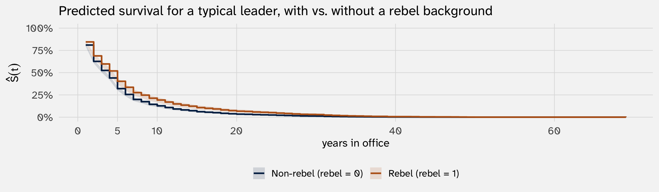
Read it: at every horizon, the rebel-background curve sits above the non-rebel curve — the HR < 1. Vertical gap at any \(t\) = the contrast in predicted survival probabilities at that horizon
Why are the curves jagged (and where do the CIs come from)?
Cox’s baseline survival \(\hat S_0(t)\) is a step function — the Breslow estimator only changes value at observed event times. Since \(\hat S(t \mid X) = \hat S_0(t)^{\exp(X\hat\beta)}\), the predicted curve is also a step function (just like KM was; very different from the smooth Exp/Weibull curves earlier, which had parametric baselines). The CI ribbons come straight from survfit() — sf_scenarios$lower and sf_scenarios$upper, computed via delta method on the cumulative hazard.
7. Competing risks: not all exits are the same
Two leaders, identical data — different stories
Suppose Leader A and Leader B both have duration = 8 and event = 1:
| Leader A | Leader B | |
|---|---|---|
| Years in office | 8 | 8 |
| Exited? | Yes | Yes |
| How they exited | Term-limited (lost re-election) | Coup (overthrown by military) |
The standard Cox model treats these as the same event. It estimates a single hazard ratio averaging across both kinds of exits
But the causes of exit are mechanistically very different. If rebel raises the risk of a coup but doesn’t change the risk of being term-limited, lumping them together averages a real effect with a zero effect — and the lumped HR understates the real coup-risk effect
Coding exit types
The leader data doesn’t record cause-of-exit, so we’ll use a coarse proxy: in established post-1950 democracies, exits are typically regular (term limits, election losses); in non-democracies, exits are typically irregular (coups, death-in-office)
# Coarse heuristic — for teaching only. Real research uses Archigos exit codes.
established_democracies_gw = c(
  2,   # USA          200, # UK           220, # France
  255, # Germany      325, # Italy        20,  # Canada
  900, # Australia    920, # New Zealand  740, # Japan
  205, # Ireland      210, # Netherlands  211, # Belgium
  225, # Switzerland  305, # Austria      350, # Greece
  375, # Finland      380, # Sweden       385, # Norway
  390, # Denmark      395, # Iceland      230, # Spain
  235                                          # Portugal
)

leader_cr = juanr::leader |>
  group_by(country, leader) |>
  summarise(
    gwcode      = first(gwcode),
    duration    = max(yr_office),
    end_year    = max(year),
    age_start   = first(age,         order_by = year),
    edu         = first(edu,          order_by = year),
    mil_service = first(mil_service, order_by = year),
    combat      = first(combat,       order_by = year),
    rebel       = first(rebel,        order_by = year),
    .groups     = "drop"
  ) |>
  mutate(event = as.integer(end_year < 2015)) |>
  drop_na(duration, age_start, mil_service, combat, rebel, edu) |>
  mutate(
    is_democracy = gwcode %in% established_democracies_gw & end_year >= 1950,
    exit_type    = case_when(
      event == 0     ~ "censored",
      is_democracy   ~ "regular",     # democracy → term limit / election loss
      !is_democracy  ~ "irregular"    # autocracy → coup / in-office death
    )
)| exit_type | n |
|---|---|
| censored | 36 |
| irregular | 2116 |
| regular | 90 |
Cause-specific Cox
The simplest competing-risks approach: fit a separate Cox model for each cause, treating other-cause exits as censored
# Regular exits (irregular exits treated as censored)
mod_cox_reg = coxph(
  Surv(duration, exit_type == "regular") ~ age_start + mil_service + combat + rebel,
  data = leader_cr
)

# Irregular exits (regular exits treated as censored)
mod_cox_irr = coxph(
  Surv(duration, exit_type == "irregular") ~ age_start + mil_service + combat + rebel,
  data = leader_cr
)
Why “censored”? If a democratic leader exits via term limit, they can no longer exit by coup — so for the irregular-exit model, that observation tells us only “they made it \(t\) years without an irregular exit.” That’s exactly censoring
Same data, three stories
| Standard Cox (lumped) | Regular exits | Irregular exits | |
|---|---|---|---|
| age_start | 1.029*** | 1.054*** | 1.028*** |
| (0.002) | (0.010) | (0.002) | |
| mil_service | 0.936 | 1.191 | 0.924 |
| (0.073) | (0.447) | (0.073) | |
| combat | 1.013 | 0.790 | 1.026 |
| (0.087) | (0.357) | (0.089) | |
| rebel | 0.799*** | 0.113*** | 0.841** |
| (0.042) | (0.059) | (0.045) | |
| Num.Obs. | 2242 | 2242 | 2242 |
| + p < 0.1, * p < 0.05, ** p < 0.01, *** p < 0.001 |
The lumped HR for rebel is an average of the cause-specific HRs, weighted by how common each exit type is. Reading the cause-specific columns separately reveals whether rebel matters for both kinds of exit, only one, or in opposite directions
Use cause-specific Cox when: you can identify distinct exit types in your data (Archigos codes for leader exits; cause-of-death codes for mortality; “left for another job” vs. “fired” in employment) AND you have theoretical reasons to think covariate effects differ across causes
Recap
Duration-model toolkit
| Question you’re asking | Right tool | Fitting method | R |
|---|---|---|---|
| What does survival look like in my data, by group? | Kaplan-Meier | Nonparametric | survfit(Surv(t, e) ~ X) |
| What’s the predicted survival time at scenario \(X\)? | Exponential / Weibull (AFT) | Full MLE | survreg(..., dist = "weibull") |
| How does \(X\) affect the hazard, holding shape free? | Cox PH | Partial likelihood | coxph(...) |
| Are different causes of exit driven by different things? | Cause-specific Cox / Fine-Gray | Partial likelihood | coxph(Surv(t, type == "k") ~ ...) |
A note on fitting: Exp/Weibull use full MLE — write the likelihood, maximize. Cox uses partial likelihood — the baseline hazard \(h_0(t)\) is never estimated; partial likelihood gives MLE-quality inference without committing to a baseline shape. Same asymptotic guarantees (consistency, asymptotic normality), different machinery
For most political-science effect-of-\(X\) questions, Cox is probably the right default