| Education | Race | Sex | Religion | Voted for Obama? |
|---|---|---|---|---|
| Bachelor | White | Male | None | no |
| High School | White | Male | None | yes |
| Bachelor | White | Male | Catholic | no |
| High School | White | Female | Catholic | no |
| Graduate | White | Female | None | yes |
| Junior College | White | Female | None | yes |
Ordered & Multinomial Models
POL 213 · Week 7
Juan F. Tellez
University of California, Davis
May 13, 2026
Housekeeping
- PS4 grades done; PS6 next
- PS7 released this week; covers ordered + multinomial
- Final-project check-in this week (office hours)
- You will present to the class on May 27th
Where we are
Seven weeks so far
Wk 1: OLS
\[Y \in \mathbb{R}\]
Continuous \(Y\)
Wk 2: Transforms
\[Y = f(X)\beta\]
You chose nonlinearity
Wk 3: Logit
\[Y \in \{0,1\}\]
Binary \(Y\)
Wk 4: MLE
glm(...) — maximize the likelihood
Wk 5: Counts
\[Y \in \{0,1,2,\ldots\}\]
Poisson, NB
Wk 6: Duration
\[Y = \text{time to event}\]
Censoring
Wk 7: Categories
\[Y \in \{1, 2, \ldots, K\}\]
Ordered & nominal
Today: same MLE engine, two more outcome types — and one structurally new ingredient → choices among many alternatives
Categorical variables are qualitative
Categorical variables are qualitative:
Two flavors of categorical outcome
With more than two levels, we have:
Ordered
The categories have a natural ordering, but the gaps between them aren’t necessarily equal
- Likert scales (strongly disagree … strongly agree)
- Approval ratings (low / medium / high)
- Conflict intensity (peace / dispute / war)
- Education attainment (less than HS / HS / college / grad)
Nominal (unordered)
The categories are distinct but there is no meaningful ranking
- Vote choice (Biden / Trump / third party)
- Protest tactic (peaceful / violent / boycott)
- Migration destination (US / Europe / stay)
- Coup outcome (success / failure / coup-proofing)
Modeling “ordered” and “nominal” outcomes look superficially similar (both are categorical) but call for different statistical machinery
1. Ordered logit
Today’s first example: support for one-party rule in Ethiopia
Survey item: “There are many ways to govern a country. Would you disapprove or approve of: only one political party is allowed to stand for election and hold office?”
| opr | age | gender | urban | edu_num |
|---|---|---|---|---|
| Strongly disapprove | 25 | female | rural | 1 |
| Disapprove | 27 | male | urban | 2 |
| Approve | 19 | female | urban | 3 |
| Strongly approve | 22 | female | urban | 4 |
The outcome has a natural ordering: “strongly approve” > “approve” > “disapprove” > “strongly disapprove”. But is the gap from “disapprove → approve” the same size as from “approve → strongly approve”? Probably not
What the ordered outcome looks like
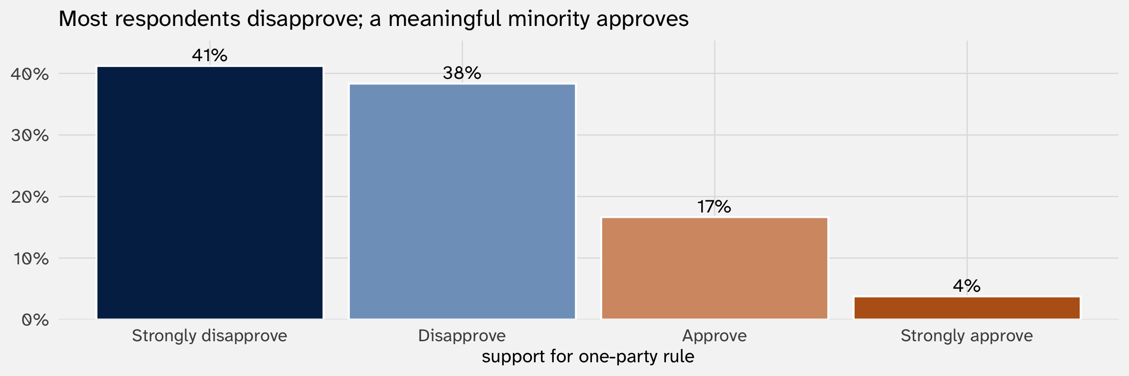
Substantive question: who supports one-party rule in Ethiopia? Treatment: education
What if we just use OLS?
The ordered outcome looks like a number (1, 2, 3, 4). What’s the harm in regressing it?
| OLS on opr (1–4) | |
|---|---|
| (Intercept) | 2.019*** |
| (0.071) | |
| age | 0.001 |
| (0.001) | |
| gendermale | −0.061+ |
| (0.036) | |
| urbanurban | 0.013 |
| (0.043) | |
| edu_num | −0.097*** |
| (0.021) | |
| Num.Obs. | 2305 |
| R2 | 0.016 |
| + p < 0.1, * p < 0.05, ** p < 0.01, *** p < 0.001 |
- Remember, OLS is giving us the conditional / expected value of Y given X
- So a one unit increase in education \(\approx\) .1 decrease on a 4-point scale
Three problems with this
1. The numbers 1–4 are arbitrary labels. We could have coded “Strongly disapprove = 1, Disapprove = 2, Approve = 3, Strongly approve = 4” or “1, 2, 7, 100” — OLS treats them as if they have meaningful spacing. The data contain less information than we’re pretending
2. The slope on education inherits that arbitrary scale. \(\hat\beta_{\text{edu}} = -0.1\) reads as “moving up one step in education shifts support down by 0.1 categories.” But what’s a “category”? OLS is treating “Strongly disapprove → Disapprove” as the same distance as “Approve → Strongly approve” — and our slope is denominated in that unit. Change the coding to (1, 2, 7, 100) and the slope changes too
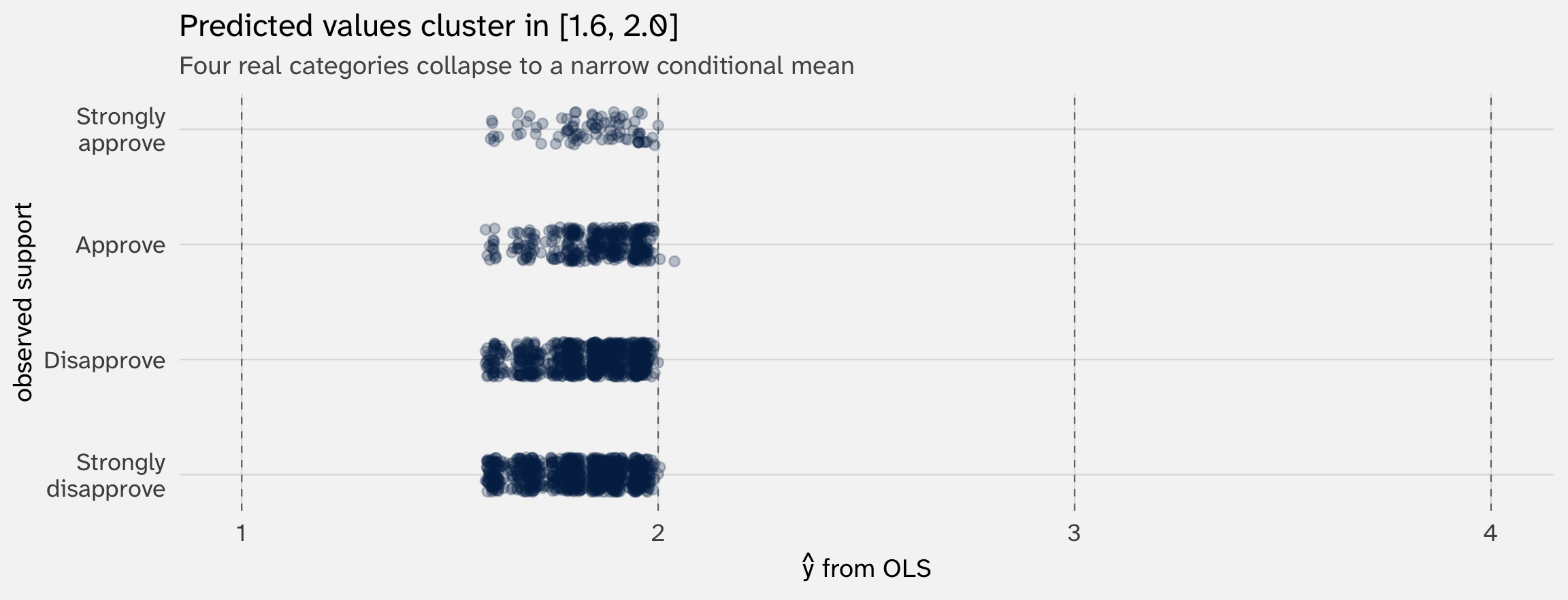
3. OLS does not mimic the DGP. For each respondent, OLS returns a single \(\hat y\) (a conditional mean, like \(1.8\)). What we might really want for an ordered outcome is a probability for each category — e.g., “60% chance of strongly disapproving, 25% disapproving, 10% approving, 5% strongly approving.” OLS can’t produce that; it collapses the whole distribution into one number
OLS gives us conditional means
# A tibble: 5 × 3
  opr_num edu_num .fitted
    <dbl>   <dbl>   <dbl>
1       2       2    1.80
2       1       1    1.94
3       2       3    1.75
4       3       3    1.76
5       1       1    1.88
Each respondent gets a single \(\hat y\) — and those \(\hat y\) values bunch tightly around the sample mean, far from the extreme categories
Same flavor of problem as: OLS on a binary outcome predicting \(\hat p > 1\). Familiar from Week 3
A different way to see Week 3’s binary logit
In Week 3 you fit a binary logit and read it as:
\[p_i \;=\; \Pr(Y_i = 1 \mid X_i) \;=\; \sigma(X_i\beta)\]
Reframe: a binary logit picks one cut on the outcome (\(Y=1\) vs \(Y=0\)) and models the probability that \(Y_i\) lies above that cut. With binary \(Y\) there’s only one possible cut
The operation generalizes: “pick a cut, model the probability of being above it” is a move we can repeat. With ordered \(Y\), there’s more than one cut to pick
What if \(Y\) has 4 ordered categories?
Our outcome opr has 4 levels: Strongly disapprove < Disapprove < Approve < Strongly approve
With 4 ordered categories, there are 3 places we could put a cut:
- Cut 1: Strongly disapprove vs. anything else
- Cut 2: Disapprove or below vs. Approve or above
- Cut 3: Anything below Strongly approve vs. Strongly approve
Each cut turns the 4-category outcome into a binary one. So a perfectly reasonable first move: just run 3 binary logits, one per cut
Where this goes: ordered logit is what we get when we tie those 3 binary logits together with one shared slope. Let’s build up to it
Where we’re headed
We want a model that:
- Handles \(J\) ordered categories (not just 2)
- Returns a probability for each category
- Respects the ordering — doesn’t pretend “Strongly disapprove” and “Strongly approve” are interchangeable
- Collapses back to binary logit when \(J = 2\)
Proportional odds assumption We are also going to assume that the slope of any explanatory variable is the same across all categories → other models can relax this assumption
Try it: stack three binary logits
Build three binary outcomes from opr, one per cut, and fit each with glm. Use a numeric education score 1–4 so each model has one slope on edu_num
# Cut 1: is Y ≥ Disapprove? (anything but strongly disapprove)
mod_b1 = glm(opr_num >= 2 ~ edu_num + age + gender + urban,
             data = afro, family = binomial)

# Cut 2: is Y ≥ Approve?
mod_b2 = glm(opr_num >= 3 ~ edu_num + age + gender + urban,
             data = afro, family = binomial)

# Cut 3: is Y = Strongly approve?
mod_b3 = glm(opr_num >= 4 ~ edu_num + age + gender + urban,
             data = afro, family = binomial)
Three separate binary logits, each with its own intercept and its own slope. Each tells us \(\Pr(Y_i \ge j \mid X_i) = \sigma(X_i\beta_j + \alpha_j)\) for one cut \(j\)
What we get back
| Source | slope on edu_num | intercept |
|---|---|---|
| `glm`: Y ≥ Disapprove | -0.245 | 0.975 |
| `glm`: Y ≥ Approve | -0.219 | -1.044 |
| `glm`: Y = Strongly approve | -0.123 | -3.442 |
Two things to notice
- The three slopes are similar — they all say more education → less support for one-party rule, with roughly the same magnitude
- They aren’t identical, but the differences are small enough to be plausibly sampling noise around a single underlying \(\beta\). If that’s right, estimating three separate slopes throws away precision
- If it’s not right — the three slopes differ in a real, systematic way — pooling is the wrong move and we’d be hiding genuine heterogeneity. We’ll come back to this as the proportional-odds assumption and learn how to test it
Results differ across applications!
We are just looking at education with this afrobarometer data. Obviously, these patterns will look different in other applications
Pool the slopes: one \(\beta\), three cutpoints
The move: force the three binary logits to share a single slope \(\beta\), but let each cut keep its own intercept. Rename the intercepts as cutpoints \(\tau_1 < \tau_2 < \tau_3\):
Week 3 — binary logit
\[\Pr(Y_i = 1 \mid X_i) \;=\; \frac{1}{1 + e^{-(\beta_0 + \beta_1 X_i)}}\]
- one equation, one cut on \(Y\) (0 vs 1)
- intercept \(\beta_0\) tells you where the cut sits
- slope \(\beta_1\): effect of \(X\) on the latent index
Today — ordered logit
\[\Pr(Y_i \le j \mid X_i) \;=\; \frac{1}{1 + e^{-(\tau_j - \beta_1 X_i)}}\]
for \(j = 1, \dots, J-1\)
- \(J - 1\) equations, one per cut on \(Y\)
- cutpoints \(\tau_1 < \tau_2 < \tau_3\): one intercept per cut
- slope \(\beta_1\): same \(\beta_1\) across all cuts
The three equations, written out
For our one-party-rule outcome (\(J = 4\) categories), the model is three equations, one per cut, sharing a single \(\beta\):
\[\Pr(\text{Y} \le \text{Strongly disapprove} \mid X_i) \;=\; \sigma(\tau_1 - X_i\beta)\]
Cut 1: below this line = “strongly disapprove”; above = anything else
\[\Pr(\text{Y} \le \text{Disapprove} \mid X_i) \;=\; \sigma(\tau_2 - X_i\beta)\]
Cut 2: below this line = “strongly disapprove” or “disapprove”; above = approves of some flavor
\[\Pr(\text{Y} \le \text{Approve} \mid X_i) \;=\; \sigma(\tau_3 - X_i\beta)\]
Cut 3: below this line = anything but “strongly approve”; above = “strongly approve”
Three equations, one \(\beta\), three cutpoints (\(\tau_1 < \tau_2 < \tau_3\)). That’s the entire ordered logit specification for our four-category outcome
Per-category probabilities by subtraction
The model gives us the cumulative probability \(\Pr(Y_i \le j \mid X_i)\) at each cut. To get the probability of exactly category \(j\), subtract:
\[\Pr(Y_i = j \mid X_i) \;=\; \sigma(\tau_j - X_i\beta) - \sigma(\tau_{j-1} - X_i\beta)\]
Big picture: ordered logit = stack \(J-1\) binary logits at successive cuts, force them to share a slope, read off the per-category probabilities by differencing the cumulative ones. Nothing structurally new since Week 3
Side-by-side: Week 4’s logit log-likelihood, and today’s
Week 4 — binary logit, the log-likelihood you’ve already maximized:
\[\qquad \ell(\beta) \;=\; \sum_{i=1}^n \Bigl[\, Y_i \log \sigma(X_i\beta) + (1 - Y_i) \log(1 - \sigma(X_i\beta)) \,\Bigr]\]
Today — ordered logit, what polr maximizes:
\[\ell(\beta, \tau) \;=\; \sum_{i=1}^n \sum_{j=1}^J \mathbb{1}\{Y_i = j\} \;\log\!\bigl[\,\sigma(\tau_j - X_i\beta) - \sigma(\tau_{j-1} - X_i\beta)\,\bigr]\]
Ordered logit with J = 2 → Logit
When there are only two categories, the inner sum collapses into the familiar \(Y_i \log p_i + (1 - Y_i) \log(1 - p_i)\)
What does each respondent contribute?
For our one-party-rule outcome (\(J = 4\)), every respondent contributes only one of four terms to \(\ell(\beta, \tau)\) — the indicator \(\mathbb{1}\{Y_i = j\}\) zeros out the other three categories. Each respondent’s contribution depends on which box they checked:
Strongly disapprove
\[\log\!\bigl[\,\sigma(\tau_1 - X_i\beta) - 0\,\bigr]\]
Disapprove
\[\log\!\bigl[\,\sigma(\tau_2 - X_i\beta) - \sigma(\tau_1 - X_i\beta)\,\bigr]\]
Approve
\[\log\!\bigl[\,\sigma(\tau_3 - X_i\beta) - \sigma(\tau_2 - X_i\beta)\,\bigr]\]
Strongly approve
\[\log\!\bigl[\,1 - \sigma(\tau_3 - X_i\beta)\,\bigr]\]
Top and bottom use \(0\) and \(1\) (the implicit cutpoints \(\tau_0 = -\infty\), \(\tau_4 = +\infty\)); the middle two use σ-differences. polr finds \((\beta, \tau_1, \tau_2, \tau_3)\) that maximize the sum
Searching for \(\beta\) and the cutpoints
The log-likelihood. Plug in \(\beta\) and \((\tau_1, \tau_2, \tau_3)\), get a number — how probable the observed data is under those parameters
Heads up: to keep the code readable we’ll drop the other covariates and fit a bivariate model — \(\text{opr} \sim \text{edu\_num}\). With one \(X\), we don’t need matrix algebra
\[\ell(\beta, \tau) \;=\; \sum_{i=1}^n \log \sigma(\tau_{Y_i} - \beta\,\text{edu}_i) - \sigma(\tau_{Y_i - 1} - \beta\,\text{edu}_i)\]
Let’s write a function that calculates \(p_i\) and \(\ell\) based on the data and the parameters \((\beta, \tau_1, \tau_2, \tau_3)\):
# log-likelihood as a function of β and the three cutpoints
log_lik = function(b, t1, t2, t3) {
  # pad with ±Inf so τ_0 and τ_J are explicit:
  # tau = [ -Inf, τ_1, τ_2, τ_3, +Inf ]   in positions 1..5
  tau = c(-Inf, t1, t2, t3, Inf)
  eta = b * X                              # linear predictor (scalar × vector)
  # plogis(z) is just R's name for σ(z) = 1 / (1 + exp(-z))
  p   = plogis(tau[Y + 1] - eta) - plogis(tau[Y] - eta)
  sum(log(p))
}Plug in \((\beta, \tau)\), compute \(\ell\)
Let’s plug in polr’s estimates and compare to logLik(m_simple)
# define X (edu), Y (opr 1-4), and fit polr
X = afro$edu_num
Y = as.integer(afro$opr)
m_simple = polr(opr ~ edu_num, data = afro)

# polr's β and three cutpoints
b_hat = coef(m_simple)
tau   = m_simple$zeta

# by-hand vs polr
c(by_hand = log_lik(b_hat, tau[1], tau[2], tau[3]),
  polr    = as.numeric(logLik(m_simple)))
by_hand polr
-2642.698 -2642.698 Identical. polr is doing exactly what the formula says — σ-difference at each respondent’s observed category, log, sum. Same machinery as Week 4, just more terms because the outcome has more categories
Fitting the full model: MASS::polr
| OLS on opr (1–4) | Ordered logit | |
|---|---|---|
| age | 0.001 | 0.001 |
| (0.001) | (0.003) | |
| gendermale | −0.061+ | −0.163* |
| (0.036) | (0.080) | |
| urbanurban | 0.013 | 0.006 |
| (0.043) | (0.096) | |
| edu_num | −0.097*** | −0.234*** |
| (0.021) | (0.047) | |
| Num.Obs. | 2305 | 2305 |
| R2 | 0.016 | |
| + p < 0.1, * p < 0.05, ** p < 0.01, *** p < 0.001 | ||
| Cutpoints (τ) and OLS intercept omitted |
Reading the coefficients
- Coefficients are on the ordered log-odds scale, same as Week 3 — but it’s the log of cumulative odds: \(\beta\) shifts \(\log\!\bigl[\Pr(Y > j) / \Pr(Y \le j)\bigr]\) by the same amount at every cut \(j\) (that’s “proportional odds”)
- expected change in the log-odds of being in a higher category versus a lower category for a one-unit increase in the predictor
- Sign reads like Week 3: \(\hat\beta_{\text{edu}} < 0\) → more education shifts probability mass into lower categories
- Interpret using same tools from Week 3
How similar is polr to the stacked logits?
Compare polr single \(\beta\) — and its three cutpoints — against the three stacked binary logits from earlier:
| Source | slope on edu_num | cutpoint / −intercept |
|---|---|---|
| `polr` (ordered logit) | -0.234 | τ = (-0.85, 0.89, 2.78) |
| `glm`: Y ≥ Disapprove | -0.245 | −α = -0.97 |
| `glm`: Y ≥ Approve | -0.219 | −α = 1.04 |
| `glm`: Y = Strongly approve | -0.123 | −α = 3.44 |
What this shows:
polr’s single \(\beta\) sits inside the spread of the three separate binary slopes, and its cutpoints \(\tau\) are in the neighborhood of the negated binary intercepts — but not identical- The third cut drifts most (\(\tau_3 = 2.78\) vs \(-\alpha = 3.44\)), the same place the third binary slope drifts. That’s proportional odds holding only approximately — we’ll come back to it
Predicted probabilities by hand — one category
Let’s compute Pr(Approve) ourselves at each education level, using mod_ord. “Approve” is the middle-upper category, so the formula uses both cutpoints:
\[\Pr(Y_i = \text{Approve} \mid X_i) \;=\; \sigma(\tau_3 - X_i\beta) - \sigma(\tau_2 - X_i\beta)\]
By hand
b = coef(mod_ord)
t = mod_ord$zeta              # τ_1, τ_2, τ_3

# linear predictor for a "typical" respondent:
xb = b["edu_num"] * 1:4 + b["gendermale"]*0 + b["urbanurban"]*0 +
     b["age"] * mean(afro$age)

# Pr(Approve) = σ(τ_3 − Xβ) − σ(τ_2 − Xβ)
pr_approve = plogis(t[3] - xb) -
             plogis(t[2] - xb)
round(pr_approve, 3)
[1] 0.206 0.174 0.145 0.120Via marginaleffects
# A tibble: 4 × 2
  edu_num estimate
    <int>    <dbl>
1       1    0.206
2       2    0.174
3       3    0.145
4       4    0.120
Why not crossing() + augment()?
predict() and augment() return the data in less plot-friendly format than predictions()
Predicted probabilities across education
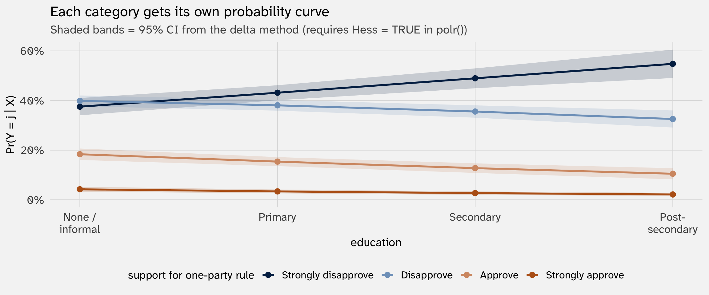
Education shifts people away from approval of “one party rule” and towards opposition
Average marginal effects (AMEs)
The marginal effect of \(X\) on \(\Pr(Y_i = j)\) is the derivative of the σ-difference w.r.t. \(X\):
\[\frac{\partial \Pr(Y_i = j)}{\partial X_i} \;=\; -\beta \cdot \Bigl[\,\sigma(\tau_j - X_i\beta)\bigl(1 - \sigma(\tau_j - X_i\beta)\bigr) \;-\; \sigma(\tau_{j-1} - X_i\beta)\bigl(1 - \sigma(\tau_{j-1} - X_i\beta)\bigr)\,\Bigr]\]
Average that across the sample to get the AME. avg_slopes does it for you:
| contrast | group | estimate | std.error | p.value |
|---|---|---|---|---|
| dY/dX | Strongly disapprove | 0.056 | 0.011 | 0 |
| dY/dX | Disapprove | -0.018 | 0.004 | 0 |
| dY/dX | Approve | -0.029 | 0.006 | 0 |
| dY/dX | Strongly approve | -0.008 | 0.002 | 0 |
Each row says: averaging across the sample, a one-step increase in education changes the probability of falling in category \(j\) by this much. The four numbers sum to zero (probability has to come from somewhere)
Why “equal gaps” is the real OLS problem
The coding is arbitrary. Coding \(Y\) as \(1, 2, 3, 4\) forces the outcome scale to have unit spacing — but those integers tell you nothing about how the probability mass is actually distributed across categories
Why it bites: an OLS coefficient of \(0.5\) reads as “\(X\) shifts \(Y\) by half a category.” Sounds like that could push lots of respondents up one step. But the real difficulty of crossing each threshold depends on where the categories sit on the latent line — not on the integer codes
Concretely in our data — polr’s cutpoints are \(\tau = (-0.86,\, 0.89,\, 2.78)\). They are not equally spaced:
- Gap from \(\tau_1\) to \(\tau_2\): about \(1.75\) latent units
- Gap from \(\tau_2\) to \(\tau_3\): about \(1.89\) latent units
- \(\tau_3\) sits far out at \(2.78\) because “Strongly approve” is rare — pushing mass across that threshold takes a much larger shift in \(X\beta\) than pushing mass across \(\tau_1\)
The fix: ordered logit lets the cutpoints land wherever the data put them on the latent line. Rare categories get distant cutpoints; common categories sit close to the center. Our coding choice (\(1, 2, 3, 4\) vs. \(1, 2, 7, 100\)) doesn’t change a thing — the model figures out the spacing on its own
Testing proportional odds — the Brant test
The intuition: remember the three stacked binary logits from earlier (\(Y \ge 2\), \(Y \ge 3\), \(Y \ge 4\)), each with its own slope on every covariate. polr collapsed those three slopes into one shared \(\beta\) per covariate. Brant asks: was that pooling defensible?
What it compares
- Restricted model: polr’s single \(\beta\) per covariate (proportional odds imposed)
- Unrestricted model: \(J - 1\) separate \(\beta\)’s per covariate (one per cut) → the stacked logits from earlier
- Test statistic: a \(\chi^2\) measuring whether the unrestricted slopes differ from each other more than sampling noise allows
\(H_0\): all \(J-1\) slopes are equal (prop odds holds) → can’t reject = pooling is fine
The Brant test of proportional odds
--------------------------------------------
Test for    X2  df  probability
--------------------------------------------
Omnibus     16  8   0.04
edu_num     0.84    2   0.66
age     2.22    2   0.33
gendermale  2.47    2   0.29
urbanurban  5.85    2   0.05
--------------------------------------------

H0: Parallel Regression Assumption holds
Reading this output
- edu_num (\(p = 0.66\)): prop odds holds — the education slope is the same at every cut. Focal predictor is well-behaved
- age (\(p = 0.33\)), gender (\(p = 0.29\)): also fine
- urban (\(p = 0.05\)): borderline — urban/rural gap may differ across cuts
- Omnibus (\(p = 0.04\)): just rejects, driven by
urban
What to do: violation is mild and lives in a control, not our focal predictor → keep polr, note the limitation
If edu_num had failed: (a) collapse categories, or (b) generalized ordered logit (VGAM::vglm)
Your turn: a full ordered-logit workflow
Data: socviz::gss_sm. Outcome: polviews (7-point liberal–conservative). Treatment: kids (number of children, treated as numeric — as.numeric(kids))
1. Stacked binary logits: fit six binary logits, one for each cumulative cut \(Y \ge j+1\). Note the slopes on kids — are they similar across cuts?
2. Ordered logit with polr: fit polr(polviews ~ as.numeric(kids), ...). How does the pooled \(\hat\beta\) compare to the six stacked-logit slopes?
3. Predicted probabilities: use marginaleffects::predictions() to get \(\Pr(Y = j)\) at each value of kids. Plot the seven curves
4. Brant test: run brant::brant() on your polr fit. Does kids satisfy proportional odds? What about the omnibus test?
Toolkit so far
| What you have | Right tool | R |
|---|---|---|
| Continuous \(Y\) | OLS | lm() |
| Binary \(Y \in \{0,1\}\) | Logit | glm(family = binomial) |
| Counts \(Y \in \{0, 1, 2, \ldots\}\) | Poisson / NB | glm(family = poisson); MASS::glm.nb() |
| Time to event \(T \ge 0\), censored | Cox PH | survival::coxph() |
| Ordered \(Y \in \{1, \ldots, J\}\) | Ordered logit | MASS::polr() |
| Nominal \(Y\) | ? | next |
For nominal outcomes the latent-variable story breaks down — there’s no single \(y^*\) to carve up. We need one latent value per alternative
2. Multinomial logit
Today’s second example: US party identification
GSS 2016, n = 2,750 respondents. Outcome: 7-point party ID collapsed to Democrat / Independent / Republican
| partyid3 | age | sex | race | educ3 | religion4 |
|---|---|---|---|---|---|
| Independent | 47 | Male | White | BA or higher | None |
| Democrat | 61 | Male | White | HS or less | None |
| Republican | 72 | Male | White | BA or higher | Catholic |
The outcome has no clean ordering: D and R are obviously opposites on a left–right axis, but Independents aren’t necessarily a “midpoint”
What the nominal outcome looks like
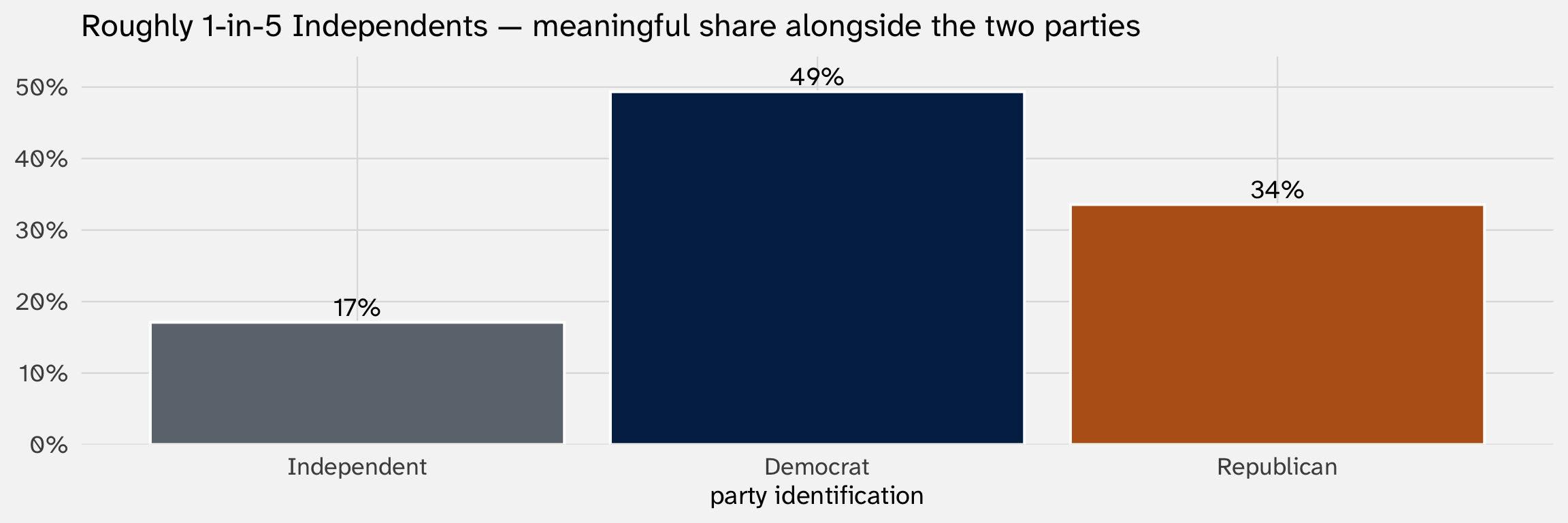
Substantive question: how does education shape who identifies as Democrat, Republican, or Independent in the modern US? Focal predictor: education (coded 1 = HS or less, 2 = Some college, 3 = BA or higher)
Same idea as ordered logit: extending Week 3 logit to \(>2\) categories
In Week 3, you fit a binary logit when the outcome had two alternatives:
\[p_i \;=\; \Pr(Y_i = 1 \mid X_i) \;=\; \sigma(X_i\beta) \;=\; \frac{1}{1 + e^{-X_i\beta}}\]
We want a model that:
- Handles \(K\) unordered alternatives (not just 2)
- Returns a probability for each that sum to 1 (\(Pr(D) + Pr(R) + Pr(I) = 1\))
- Collapses back to binary logit when \(K = 2\)
Same playbook as the ordered case: re-express the multi-category problem as a small set of binary logits, then tie them together
A different way to see Week 3’s binary logit — again
Binary logit gives us \(\Pr(Y_i = 1)\), but it works just as well to read it as a model of the log-odds of \(Y=1\) vs. \(Y=0\), with \(Y=0\) as the “baseline” category:
\[\log \frac{\Pr(Y_i = 1 \mid X_i)}{\Pr(Y_i = 0 \mid X_i)} \;=\; X_i\beta\]
Reframe: a binary logit is a model of the log-odds of one category vs. a baseline. With binary \(Y\) there’s only one such contrast to model. With more categories, there will be more
Where this goes: pick a baseline, model every other category’s log-odds against it
What if \(Y\) has 3 unordered categories?
Our outcome partyid3 has 3 levels: Democrat / Independent / Republican. Unordered — there’s no natural way to rank them, so the ordered-logit cutpoint trick won’t work
But the “pick a baseline, build binary contrasts” idea does:
- Pick a baseline category. Say Independent.
- Build \(K-1 = 2\) contrasts against that baseline:
- Democrat vs. Independent
- Republican vs. Independent
Each contrast is a binary logit on the subset where \(Y\) is in one of those two categories. So a natural first move: just run 2 binary logits
Does the choice of baseline matter?
In a narrow sense, yes: your coefficients tell you about changes in probability away from that baseline. But for inference, no, predicted probabilities and AMEs will not depend on choice of baseline.
Try it: run two binary logits
# Democrat vs. Independent — drop Republicans
mod_di = glm(I(partyid3 == "Democrat") ~ educ_num + age + sex + race + religion4,
             data   = filter(gss, partyid3 != "Republican"),
             family = binomial)

# Republican vs. Independent — drop Democrats
mod_ri = glm(I(partyid3 == "Republican") ~ educ_num + age + sex + race + religion4,
             data   = filter(gss, partyid3 != "Democrat"),
             family = binomial)
Two separate binary logits, two sets of coefficients. Each one is interpreted relative to Independent — the same way Week 3 coefficients were interpreted relative to \(Y=0\)
What we get back
| Contrast | slope on educ_num | intercept | subsample n |
|---|---|---|---|
| `glm`: Democrat vs. Independent | 0.394 | -0.822 | 1827 |
| `glm`: Republican vs. Independent | 0.340 | 0.045 | 1393 |
Two things to notice
- Both education slopes are positive — more educated respondents are more likely to identify as Dem or as Rep (relative to Independent). Unlike ordered logit, the two slopes are free to differ in magnitude — and they do (0.39 vs. 0.34). No “proportional odds” claim is being defended here
- Each fit uses a different subsample. The Dem-vs-Ind model never saw a Republican; the Rep-vs-Ind model never saw a Democrat
Why not stop here?
Running \(K-1\) models seems reasonable. So why bother with a unified model?
Two reasons
- Each contrast uses a different subsample → throws away information. A unified fit uses everyone simultaneously → e.g., more info on controls
- The probabilities don’t have to sum to 1. We want to answer ““what’s the chance this person is a Democrat?”, not “among non-Republicans, what’s the chance this person is a Democrat?”.
- Each binary logit gives \(\Pr(\text{Dem} \mid \text{not Rep})\) and \(\Pr(\text{Rep} \mid \text{not Dem})\) — different conditioning sets. Combining them into three probabilities that sum to 1 requires extra glue
Contrast with ordered logit: there we pooled the three binary slopes into one shared \(\beta\) (proportional odds). Here we keep all \(K-1\) slopes separate — there’s no reason to expect age to affect Dem-vs-Ind the same way it affects Rep-vs-Ind. The “tying together” is only about (a) using all the data and (b) probabilities summing to 1
Pool the data, keep the slopes separate
The move: pick a baseline (say Independent, \(\beta_{\text{Ind}} = 0\)). For every other category, write down its log-odds against the baseline:
Week 3 — binary logit
\[\log \frac{\Pr(Y_i = 1)}{\Pr(Y_i = 0)} \;=\; \beta_0 + \beta_1 X_i\]
- one contrast (1 vs. 0)
- one intercept, one slope
- \(Y = 0\) is the baseline
Today — multinomial logit
\[\log \frac{\Pr(Y_i = k)}{\Pr(Y_i = K)} \;=\; \beta_{0,k} + \beta_{1,k} X_i\]
for \(k = 1, \dots, K-1\)
- \(K - 1\) contrasts (one per non-baseline category)
- \(K - 1\) separate intercepts and separate slopes
- baseline category \(K\) has \(\beta_K = 0\)
Where the unification happens: we fit all \(K-1\) contrasts jointly on the full sample, and force \(\sum_k \Pr(Y_i = k) = 1\) via the softmax denominator (the algebra of how that normalization works is in the extras deck)
The two equations, written out
For our party-ID outcome (\(K = 3\) categories, baseline = Independent), the model is two log-odds equations, one per non-baseline category, with \(\beta_{\text{Ind}} = 0\):
\[\log \frac{\Pr(Y_i = \text{Democrat})}{\Pr(Y_i = \text{Independent})} \;=\; X_i\beta_{\text{Dem}}\]
How does \(X\) change the relative odds of identifying as Dem vs. Ind?
\[\log \frac{\Pr(Y_i = \text{Republican})}{\Pr(Y_i = \text{Independent})} \;=\; X_i\beta_{\text{Rep}}\]
How does \(X\) change the relative odds of identifying as Rep vs. Ind?
Two equations, two separate sets of slopes. The full softmax just rolls these up so the three probabilities (Dem, Ind, Rep) sum to 1 at every \(X_i\)
Searching for the two \(\beta\) vectors
The log-likelihood is just a function we evaluate. Plug in \(\beta_{\text{Dem}}\) and \(\beta_{\text{Rep}}\), get a number — how probable the observed party-ID data is under those parameters
Heads up: as with ordered logit, we’ll fit a bivariate model — partyid3 ~ educ_num — so each linear predictor is just \(\beta_0 + \beta_1 \cdot \text{educ}\), no matrices
\[\ell(\beta_{\text{Dem}}, \beta_{\text{Rep}}) \;=\; \sum_{i=1}^n \log\!\left[\,\frac{\exp(X_i\beta_{Y_i})}{1 + \exp(X_i\beta_{\text{Dem}}) + \exp(X_i\beta_{\text{Rep}})}\,\right]\]
where \(X_i\beta_{Y_i}\) is the linear predictor for their observed party (or \(0\) if they’re Independent, since \(\beta_{\text{Ind}} = 0\))
# log-likelihood as a function of the four parameters
# (intercept + educ slope, separately for Dem and Rep; Ind is baseline)
log_lik = function(b0_d, b1_d, b0_r, b1_r) {
  eta_d = b0_d + b1_d * X            # linear predictor for Dem
  eta_r = b0_r + b1_r * X            # linear predictor for Rep
  # softmax denominator: Ind contributes exp(0) = 1
  denom = 1 + exp(eta_d) + exp(eta_r)
  # probability of each respondent's observed category
  p = ifelse(Y == 1, 1          / denom,
      ifelse(Y == 2, exp(eta_d) / denom,
                     exp(eta_r) / denom))
  sum(log(p))
}
Plug in \((\beta_{\text{Dem}}, \beta_{\text{Rep}})\), compute \(\ell\)
Plug in multinom’s estimates and compare to logLik(m_simple_mn):
# define X (educ_num) and Y (partyid3 as 1=Ind, 2=Dem, 3=Rep), fit multinom
X = gss$educ_num
Y = as.integer(gss$partyid3)
m_simple_mn = multinom(partyid3 ~ educ_num, data = gss, trace = FALSE)

# multinom's coefficients (2 × 2 matrix)
b = coef(m_simple_mn)

# by-hand vs multinom
c(by_hand  = log_lik(b["Democrat",  "(Intercept)"],
                     b["Democrat",  "educ_num"],
                     b["Republican","(Intercept)"],
                     b["Republican","educ_num"]),
  multinom = as.numeric(logLik(m_simple_mn)))
by_hand multinom
-2776.943 -2776.943 Fitting it: nnet::multinom
| y.level | term | estimate | std.error |
|---|---|---|---|
| Democrat | (Intercept) | -0.799 | 0.225 |
| Democrat | educ_num | 0.396 | 0.067 |
| Democrat | age | 0.017 | 0.003 |
| Democrat | sexFemale | 0.162 | 0.111 |
| Democrat | raceBlack | 0.750 | 0.147 |
| Democrat | raceOther | 0.153 | 0.179 |
| Democrat | religion4Catholic | 0.372 | 0.149 |
| Democrat | religion4None | 0.237 | 0.141 |
| Democrat | religion4Other | 0.271 | 0.208 |
| Republican | (Intercept) | 0.118 | 0.234 |
| Republican | educ_num | 0.375 | 0.071 |
| Republican | age | 0.015 | 0.003 |
| Republican | sexFemale | -0.321 | 0.119 |
| Republican | raceBlack | -1.603 | 0.207 |
| Republican | raceOther | -0.517 | 0.205 |
| Republican | religion4Catholic | -0.385 | 0.154 |
| Republican | religion4None | -1.214 | 0.161 |
| Republican | religion4Other | -1.111 | 0.247 |
Reading the coefficients
- Each row is a category vs. Independent contrast —
multinomreturns two sets, one for Dem-vs-Ind and one for Rep-vs-Ind - Coefficients are log relative-risk ratios: \(\hat\beta_{\text{educ}}^{\text{Dem}} = 0.40\) means a one-step bump in education raises the log of \(\Pr(\text{Dem})/\Pr(\text{Ind})\) by \(0.40\). \(\exp(0.40) \approx 1.49\) → a 49% jump in the odds of identifying as Dem vs. Ind
How similar is multinom to the stacked binary logits?
We fit two binary logits earlier (mod_di, mod_ri). Now compare multinom’s two sets of slopes — and intercepts — against those:
| Contrast | glm slope on educ_num | multinom slope on educ_num | glm intercept | multinom intercept |
|---|---|---|---|---|
| Dem vs. Ind | 0.394 | 0.396 | -0.822 | -0.799 |
| Rep vs. Ind | 0.340 | 0.375 | 0.045 | 0.118 |
Dem-vs-Ind is essentially identical (\(0.394\) vs \(0.396\)): multinom adds nothing the binary logit didn’t have for that contrast
Rep-vs-Ind drifts (\(0.340 \to 0.375\)): multinom’s unified fit also sees the Democrats through the softmax denominator, refining the Rep-vs-Ind contrast in ways mod_ri couldn’t (it dropped them)
Contrast with ordered logit: there, polr constrained its single \(\beta\) to be the same across cuts. Here, multinom keeps two separate slopes — the unification is only about using everyone in one likelihood, not about pooling effects
These coefficients are hard to read
multinom returns two sets of coefficients — one for “Democrat vs. Independent” and one for “Republican vs. Independent”
The raw \(\hat\beta\) are log relative-risk ratios: \(\log[\Pr(\text{Democrat}) / \Pr(\text{Independent})] = X\beta_{\text{Democrat}}\). Nobody thinks in these units
Don’t try. Reach for predicted probabilities and AMEs, exactly like ordered logit
Predicted probabilities by hand — one category
Let’s compute Pr(Democrat) ourselves at each education level, using mod_mn. The softmax formula with baseline = Independent (\(\beta_{\text{Ind}} = 0\), so \(\exp(0) = 1\)):
\[\Pr(Y_i = \text{Dem}) \;=\; \frac{\exp(X_i\beta_{\text{Dem}})}{1 + \exp(X_i\beta_{\text{Dem}}) + \exp(X_i\beta_{\text{Rep}})}\]
By hand
b = coef(mod_mn)            # 2 × 10 matrix
edus = 1:3                   # HS / Some college / BA+

# linear predictor at each education level, with
# age at the mean and other covariates at baseline
# (male, white, Protestant → those dummies are 0)
eta_dem = b["Democrat",   "(Intercept)"] +
          b["Democrat",   "educ_num"] * edus +
          b["Democrat",   "age"] * mean(gss$age)
eta_rep = b["Republican", "(Intercept)"] +
          b["Republican", "educ_num"] * edus +
          b["Republican", "age"] * mean(gss$age)

# softmax denominator (Ind contributes exp(0) = 1)
denom = exp(0) + exp(eta_dem) + exp(eta_rep)

pr_dem = exp(eta_dem) / denom
round(pr_dem, 3)
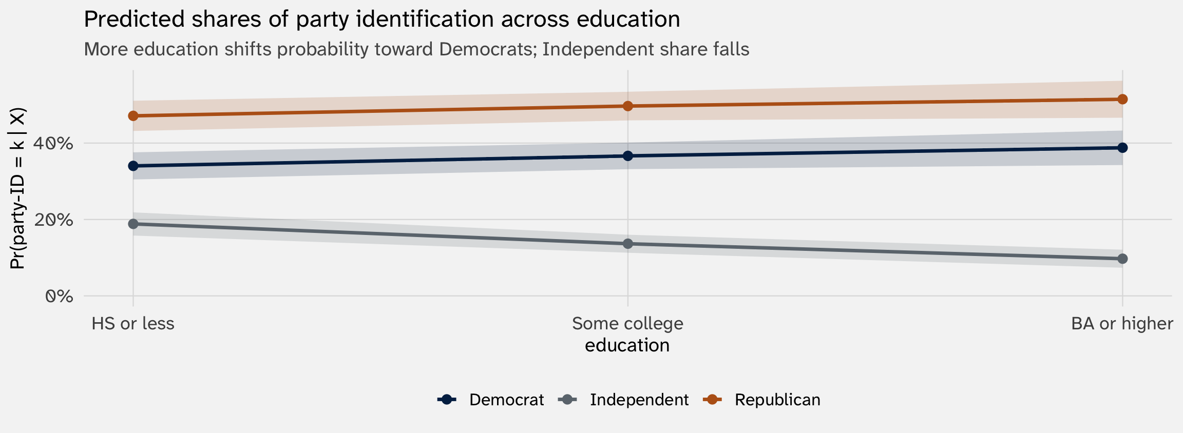
[1] 0.257 0.275 0.290Via marginaleffects
# A tibble: 3 × 2
  educ_num estimate
     <int>    <dbl>
1        1    0.257
2        2    0.275
3 3 0.29 Predicted shares across education
Average marginal effects per category
| contrast | group | estimate | std.error | p.value |
|---|---|---|---|---|
| dY/dX | Independent | -0.053 | 0.009 | 0.000 |
| dY/dX | Democrat | 0.036 | 0.010 | 0.000 |
| dY/dX | Republican | 0.017 | 0.009 | 0.068 |
Each row says: averaging across the sample, a one-step increase in education changes the probability of identifying with party \(k\) by this much. The three numbers sum to zero — probability has to come from somewhere
The IIA assumption
What multinomial logit assumes about choices
\[\frac{\Pr(Y = k)}{\Pr(Y = \ell)} = \frac{\exp(X\beta_k)}{\exp(X\beta_\ell)} = \exp\!\big(X(\beta_k - \beta_\ell)\big)\]
The ratio between any two alternatives’ probabilities depends only on the parameters of those two alternatives — not on what other options exist. This is the Independence of Irrelevant Alternatives (IIA) assumption
A property of the model, not of the world: IIA is an algebraic consequence of the softmax form
When IIA fails: the red-bus / blue-bus problem
Imagine commuting choices: drive a car, take a red bus
Suppose people pick 50/50 → \(\Pr(\text{car}) = \Pr(\text{red bus}) = 0.5\)
Now we add a blue bus that is identical to the red bus in every way except the color
What should happen? The 50% who take the bus should split between red and blue → \(\Pr(\text{car}) = 0.5\), \(\Pr(\text{red}) = \Pr(\text{blue}) = 0.25\)
What multinomial logit predicts under IIA: every alternative gets equal share → \(\Pr(\text{car}) = \Pr(\text{red}) = \Pr(\text{blue}) = 1/3\). Wrong
Testing IIA: drop Independents and refit
The test: fit the model on the full data (3-way: D, I, R), then refit on the Dem+Rep subsample only (2-way). Compare the Dem-vs-Rep coefficients across the two fits
The logic: IIA says \(\beta_{\text{Ind}}\) should cancel out of the Dem-vs-Rep ratio. So if the softmax is right for these data, the Dem-vs-Rep contrast should be the same whether or not Independents are in the fit
This is a model check, not a causal claim. We’re not asking what Democrats would do if Independents didn’t exist as an option — we have no way to know. We’re asking whether the parametric form gives consistent answers across subsets. Formal name: Hausman–McFadden test (1984)
gss_3way_r = gss |> mutate(partyid3 = relevel(partyid3, ref = "Republican"))
gss_2way_r = gss |> filter(partyid3 != "Independent") |>
  mutate(partyid3 = droplevels(partyid3),
         partyid3 = relevel(partyid3, ref = "Republican"))

mod_mn_3way_r = multinom(partyid3 ~ educ_num + age + sex + race + religion4,
                         data = gss_3way_r, trace = FALSE)
mod_mn_2way_r = multinom(partyid3 ~ educ_num + age + sex + race + religion4,
                         data = gss_2way_r, trace = FALSE)
Is a two-way multinomial simply a logit?
Yes! Where 1 = Democrat, 0 = Republican.
Comparing the two
| term | 3-way (D, I, R) | 2-way (D, R only) |
|---|---|---|
| (Intercept) | -0.917 (0.191) | -0.960 (0.194) |
| educ_num | 0.021 (0.050) | 0.023 (0.051) |
| age | 0.002 (0.003) | 0.002 (0.003) |
| sexFemale | 0.482 (0.093) | 0.487 (0.095) |
| raceBlack | 2.353 (0.177) | 2.421 (0.179) |
| raceOther | 0.670 (0.166) | 0.683 (0.167) |
| religion4Catholic | 0.758 (0.115) | 0.798 (0.116) |
| religion4None | 1.451 (0.133) | 1.524 (0.135) |
| religion4Other | 1.382 (0.199) | 1.444 (0.200) |
Formal test (Hausman–McFadden): We can use mlogit::hmftest(). The function expects mlogit-format data (one row per (respondent × alternative) pair) and two fits — one on the full choice set, one on a subset — and tests whether the shared coefficients agree
# Reshape to mlogit long format
gss_ml = mlogit.data(gss, choice = "partyid3", shape = "wide")

# Full and restricted fits (drop Independent in the restricted)
m_full = mlogit(partyid3 ~ 0 | educ_num + age + sex + race + religion4,
                data = gss_ml, reflevel = "Republican")
m_red  = mlogit(partyid3 ~ 0 | educ_num + age + sex + race + religion4,
                data = gss_ml, reflevel = "Republican",
                alt.subset = c("Republican", "Democrat"))

hmftest(m_full, m_red)
    Hausman-McFadden test

data:  gss_ml
chisq = 12.119, df = 9, p-value = 0.2067
alternative hypothesis: IIA is rejected
Reading it: \(p \approx 0.21\) — can’t reject IIA. The Dem-vs-Rep contrast is statistically the same whether we fit on all three categories or just (D, R). softmax is a defensible fit for these data
How worried should we be?
The Democrat-vs-Republican coefficients are broadly similar in the 3-way and 2-way models — IIA looks like a defensible approximation here
What kinds of choice sets are suspicious? The common thread is unobserved similarity — features of the alternatives that the model can’t see, so they share structure invisibly:
- Close substitutes (red bus / blue bus): alternatives that share unmeasured attributes — like “is a bus” — won’t be treated as substitutes by the softmax. The shared attribute is invisible to the model
- Ideologically-clustered alternatives (Left / Center / Right candidates): alternatives that lie on a latent similarity dimension the model doesn’t measure
- Spatial alternatives (neighborhoods, retail stores): alternatives clustered in geographic or feature space, sharing proximity attributes the model isn’t conditioning on
When IIA fails, other options: nested logit (group similar alternatives), mixed logit (let preferences vary across people), conditional logit with alternative-specific covariates
Toolkit, updated
| What you have | Right tool | R |
|---|---|---|
| Continuous \(Y\) | OLS | lm() |
| Binary \(Y \in \{0,1\}\) | Logit | glm(family = binomial) |
| Counts \(Y \in \{0, 1, \ldots\}\) | Poisson / NB | glm(family = poisson); MASS::glm.nb() |
| Time to event \(T \ge 0\), censored | Cox PH | survival::coxph() |
| Ordered \(Y \in \{1, \ldots, J\}\) | Ordered logit | MASS::polr() |
| Nominal \(Y \in \{1, \ldots, K\}\) | Multinomial logit | nnet::multinom() |