Prediction & Machine Learning
POL 213 · Week 8
University of California, Davis
May 20, 2026
Housekeeping
- Project presentations next week (May 27) — see syllabus for the rubric
- Final exam June 3
Two paths
Which way?
The economist
Identify a treatment effect — get \(\hat\beta\) right.
- Key question: what’s the effect of \(X\) on \(Y\)?
- Worry list: confounding, selection, identification
- Holds \(\hat\beta\) to a high standard; doesn’t much care about \(\hat y\)
The Statistician™
Model the data-generating process — get \(\hat y\) right.
- Key question: how well do we predict \(Y\) from \(X\)?
- Worry list: predictive performance, overfitting
- Holds \(\hat y\) to a high standard; doesn’t much care about any particular \(\hat\beta\)
Both traditions have homes1. They’re not necessarily in competition → they’re answering different questions
Two paths forward from here
For the end of the course, we’ll walk down each of these paths (for a little bit)
Statistician’s path → prediction & ML
If you care about getting \(\hat y\) right, the natural next step is to ask “how well do I predict?” and “can I do better?”
- Formal predictive metrics (today)
- Sacrifice linear-in-parameters → machine learning (today)
That’s this week (and a separate course!)
Economist’s path → causal inference
If you care about \(\hat\beta\) as a treatment effect, the natural next step is “what assumptions justify reading \(\hat\beta\) causally, and what other tools help?”
- Potential outcomes & identification
- Selection on observables (g-computation, IPW)
- Selection on unobservables (IV, RDD)
That’s next week (and a separate course!)
Where we are
We’ve spent seven weeks building MLE models for different kinds of outcomes:
| Week | Outcome type | Model | What goes inside |
|---|---|---|---|
| 3 | Binary \(Y \in \{0, 1\}\) | Logit | \(\sigma(X\beta)\) |
| 5 | Counts \(Y \in \{0, 1, 2, \ldots\}\) | Poisson / NB | \(\exp(X\beta)\) |
| 6 | Time-to-event \(T \ge 0\) | Cox / Weibull | \(h_0(t)\exp(X\beta)\) |
| 7 | Ordered + nominal \(Y\) | Ordered + multinomial logit | \(\sigma(\tau_j - X\beta)\) etc. |
Two things every row has in common:
- The model produces \(\hat y\) on the right scale for the outcome (in \([0,1]\), \(\ge 0\), etc.). MLE’s original job
- Each one is built around a linear-in-parameters core, \(X\beta\). The link function wraps it; the inside is always \(\beta_0 + \beta_1 X_1 + \beta_2 X_2 + \ldots\)
Today’s question
Statistician wants to faithfully model the Data Generating Process (DGP); how do we know if we’re doing that well?
Prediction: if our models’ \(\widehat{Y}\) predicts \(Y\) well, we’re on the right track
Three sections today:
- Defining “well.” Predictive performance has different definitions for different outcome types. For continuous \(Y\): MSE and \(R^2\). For binary \(Y\): ROC curves and AUC
- Honest measurement. Computing these metrics on the same data you used to fit your model has limited value. The honest version: out-of-sample evaluation.
- What if we relax linear-in-parameters? All our models had a linear-in-paramters core (\(X\beta\)). Machine-learning models drop the \(X\beta\) scaffold entirely and let \(\hat y = f(X)\) for whatever \(f\) the data want. They often (?) predict better. The cost they pay is interpretability
1a. Measuring predictive performance
How good is \(\hat Y\)?
A recurring example: V-Dem mobilization
We’ll use the same V-Dem data we worked with in Week 2:
| OLS (quadratic in democracy) | |
|---|---|
| (Intercept) | −2.754*** |
| (0.055) | |
| poly(democracy, 2, raw = TRUE)1 | 7.676*** |
| (0.177) | |
| poly(democracy, 2, raw = TRUE)2 | −8.032*** |
| (0.195) | |
| ln_gdppc | −0.044*** |
| (0.013) | |
| ln_pop | 0.179*** |
| (0.006) | |
| Num.Obs. | 11400 |
| R2 | 0.213 |
| + p < 0.1, * p < 0.05, ** p < 0.01, *** p < 0.001 |
How wrong is \(\hat y\)?
For each country-year \(i\), we have a prediction \(\hat y_i\) and a true value \(y_i\). The “mistake” is \(y_i - \hat y_i\) — the residual.
# A tibble: 6 × 10
mobilization .fitted .resid poly(democracy, 2, raw =…¹ ln_gdppc ln_pop .hat
<dbl> <dbl> <dbl> <dbl> <dbl> <dbl> <dbl>
1 -0.942 -0.246 -0.696 0.193 1.89 7.84 1.97e-4
2 -0.844 -0.236 -0.608 0.194 1.91 7.88 2.00e-4
3 -0.844 -0.231 -0.613 0.194 1.93 7.91 2.03e-4
4 -0.844 -0.216 -0.628 0.196 1.97 7.95 2.06e-4
5 -0.844 -0.210 -0.634 0.196 2.02 8.00 2.11e-4
6 -0.844 -0.206 -0.638 0.196 2.05 8.03 2.15e-4
# ℹ abbreviated name: ¹`poly(democracy, 2, raw = TRUE)`[,"1"]
# ℹ 4 more variables: `poly(democracy, 2, raw = TRUE)`[2] <dbl>, .sigma <dbl>,
# .cooksd <dbl>, .std.resid <dbl>So how good is this model?
Mean squared error (MSE)
\[\boxed{\;\text{MSE} \;=\; \frac{1}{n} \sum_{i=1}^n (y_i - \hat y_i)^2\;}\]
the average squared distance between \(\hat y\) and \(y\). Same units as the variance of \(Y\). The lower, the better. Zero means perfect prediction; bigger numbers mean a worse model
MSE is in squared mobilization units. To get back to the same scale as the outcome itself, take the square root — RMSE = \(\sqrt{\text{MSE}} \approx\) 1.176: the typical prediction is off by about ±1.2 mobilization-index units
Comparing models with MSE
One nice thing about MSE: it gives us a single number per model, so we can use it to compare candidates. How does our quadratic fit compare to a simpler linear-in-democracy model?
   linear quadratic
   1.5875    1.3825
The quadratic’s MSE is lower — it fits the data better in-sample
Linear vs. quadratic on the binned data
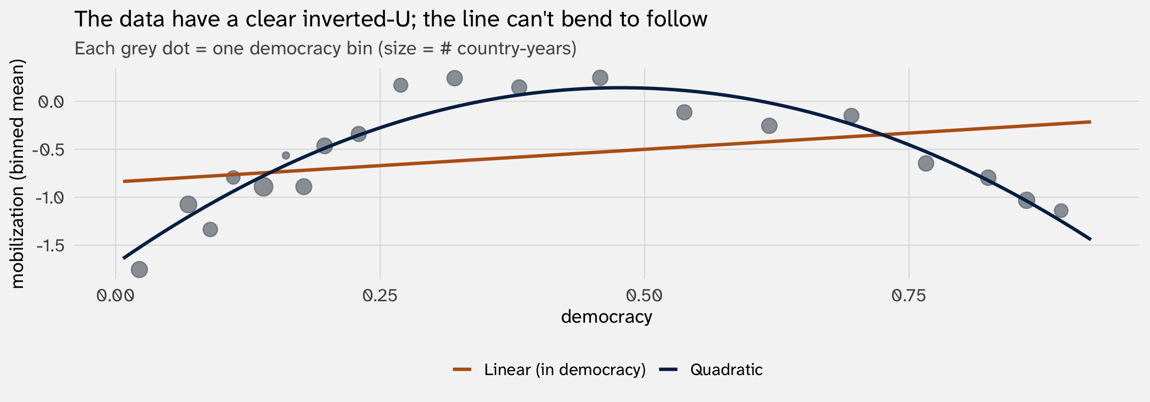
The line misses the curvature in the middle — that’s where most of its squared error comes from. The quadratic bends with the data
From MSE to R²
MSE has one nuisance: it’s in squared outcome units. “Is 1.382 big or small?” depends entirely on the scale of \(Y\)
To make MSE comparable across outcomes, divide it by the total variance of \(Y\) (which is the MSE of a null model that predicts \(\bar y\) for everyone):
\[R^2 \;=\; 1 \;-\; \frac{\text{MSE of your model}}{\text{Var}(Y)} \;=\; 1 \;-\; \frac{\text{SSR}}{\text{SST}}\]
Same \(R^2\) you’ve seen since Week 2 — just re-derived as MSE-relative-to-the-null-model. The reading is unchanged: fraction of variance explained, where 0 = no better than guessing the mean and 1 = perfect prediction
R² for both V-Dem regressions
null_mse = mean((y_obs - mean(y_obs))^2)     # = Var(Y), MSE of guessing the mean
mse_lin  = mean(residuals(mod_lin)^2)
mse_quad = mean(residuals(mod_quad)^2)

tibble(
  model = c("Linear in democracy", "Quadratic in democracy"),
  mse   = c(mse_lin, mse_quad),
  r2    = 1 - c(mse_lin, mse_quad) / null_mse
) |> mutate(across(c(mse, r2), \(x) round(x, 4)))
# A tibble: 2 × 3
model mse r2
<chr> <dbl> <dbl>
1 Linear in democracy 1.59 0.0961
2 Quadratic in democracy 1.38 0.213 So far so good — but binary outcomes ask a different question
MSE and \(R^2\) summarize squared distance between \(\hat y\) and \(y\). That’s the right thing to measure when \(y\) varies continuously
For binary \(y \in \{0, 1\}\), you can compute the same squared distance — it’s well-defined and it has a name (Brier score, \(\frac{1}{n}\sum (y_i - \hat p_i)^2\))
But the binary-Y question is usually a classification question: among the people the model thinks are most likely to support the wall, are they actually the supporters? That’s about classification, not about how close \(\hat p_i\) lands to 0 or 1 numerically
To formalize classification, we’ll use a different family of metrics built from the confusion matrix
1b. Binary outcomes: ROC and AUC
How well does the model classify positives above negatives?
Callback: the Week 3 wall-support model
In Week 3, we fit a logit predicting whether respondents in the 2020 CES support a border wall:
| Logit: support wall | |
|---|---|
| (Intercept) | −1.614*** |
| (0.032) | |
| protestantProtestant | 0.724*** |
| (0.018) | |
| age | 0.022*** |
| (0.001) | |
| sexFemale | −0.476*** |
| (0.018) | |
| newsintSome of the time | 0.267*** |
| (0.022) | |
| newsintOnly now and then | 0.324*** |
| (0.029) | |
| newsintHardly at all | 0.367*** |
| (0.037) | |
| newsintDon't know | 0.439*** |
| (0.051) | |
| Num.Obs. | 60866 |
| + p < 0.1, * p < 0.05, ** p < 0.01, *** p < 0.001 |
39.2% of respondents support the wall. The logit produces predicted probabilities \(\hat p_i \in [0, 1]\) — same model, but now we ask: how well does it predict?
From probabilities to classifications
The logit gives us \(\hat p_i\), but our outcome is a class (supporter/opponent):
# A tibble: 6 × 6
   wall protestant       age sex    newsint           .fitted
  <dbl> <fct>          <dbl> <fct>  <fct>               <dbl>
1     1 Non-Protestant    54 Male   Most of the time    0.390
2     0 Protestant        65 Female Most of the time    0.509
3     0 Protestant        74 Female Most of the time    0.557
4     0 Non-Protestant    58 Female Some of the time    0.361
5     0 Non-Protestant    53 Male   Only now and then   0.463
6     1 Protestant        59 Male   Most of the time    0.595
To turn \(\hat p_i\) into a class — predicting wall = 1 or 0 for each respondent — we have to pick a threshold \(c\) and say:
\[\hat y_i \;=\; \begin{cases} 1 & \text{if } \hat p_i > c \\ 0 & \text{otherwise} \end{cases}\]
Picking a threshold for classifying supporters
One default is \(c = 0.5\):
# A tibble: 6 × 7
   wall protestant       age sex    newsint           .fitted  pred
  <dbl> <fct>          <dbl> <fct>  <fct>               <dbl> <dbl>
1     1 Non-Protestant    54 Male   Most of the time    0.390     0
2     0 Protestant        65 Female Most of the time    0.509     1
3     0 Protestant        74 Female Most of the time    0.557     1
4     0 Non-Protestant    58 Female Some of the time    0.361     0
5     0 Non-Protestant    53 Male   Only now and then   0.463     0
6     1 Protestant        59 Male   Most of the time    0.595     1
How well did we do? The confusion matrix lets us compare each of our guesses against reality
The confusion matrix
| Predicted oppose (0) | Predicted support (1) | |
|---|---|---|
| Actually opposes (0) | True Negative (TN) | False Positive (FP) |
| Actually supports (1) | False Negative (FN) | True Positive (TP) |
Two rates we care about:
- True positive rate (TPR) = \(\frac{\text{TP}}{\text{TP} + \text{FN}}\) — of all the actual supporters, how many did we catch? (Also called sensitivity or recall)
- False positive rate (FPR) = \(\frac{\text{FP}}{\text{FP} + \text{TN}}\) — of all the actual opposers, how many did we wrongly flag as supporters?
The confusion matrix at \(c = .5\)
      predicted
actual     0     1
     0 31397  5615
1 15976 7878TPR = 0.33 — we catch 33.0% of actual supporters
FPR = 0.152 — we wrongly flag 15.2% of actual opposers
What if we lower the threshold?
More permissive? \(c = .25\)
      predicted
actual     0     1
     0  7375 29637
     1  1991 21863
TPR = 0.917 (91.7% of supporters caught) → up from 33.0%
FPR = 0.801 (80.1% of opposers wrongly flagged) → up from 15.2%
What if we raise the threshold?
More demanding? \(c = .75\)
      predicted
actual     0     1
     0 36992    20
     1 23790    64
TPR = 0.003 (0.3% of supporters caught) → down from 33.0%
FPR = 0.001 (0.1% of opposers wrongly flagged) → down from 15.2%
Lower threshold → catch more supporters (TPR up) and more false alarms (FPR up). Higher threshold → opposite. There’s no single right threshold
TPR + FPR
That’s why we focus on these two: they capture the tradeoff
ROC curve: sweep through every threshold
Instead of picking one threshold, plot TPR vs. FPR for every threshold from 0 to 1:
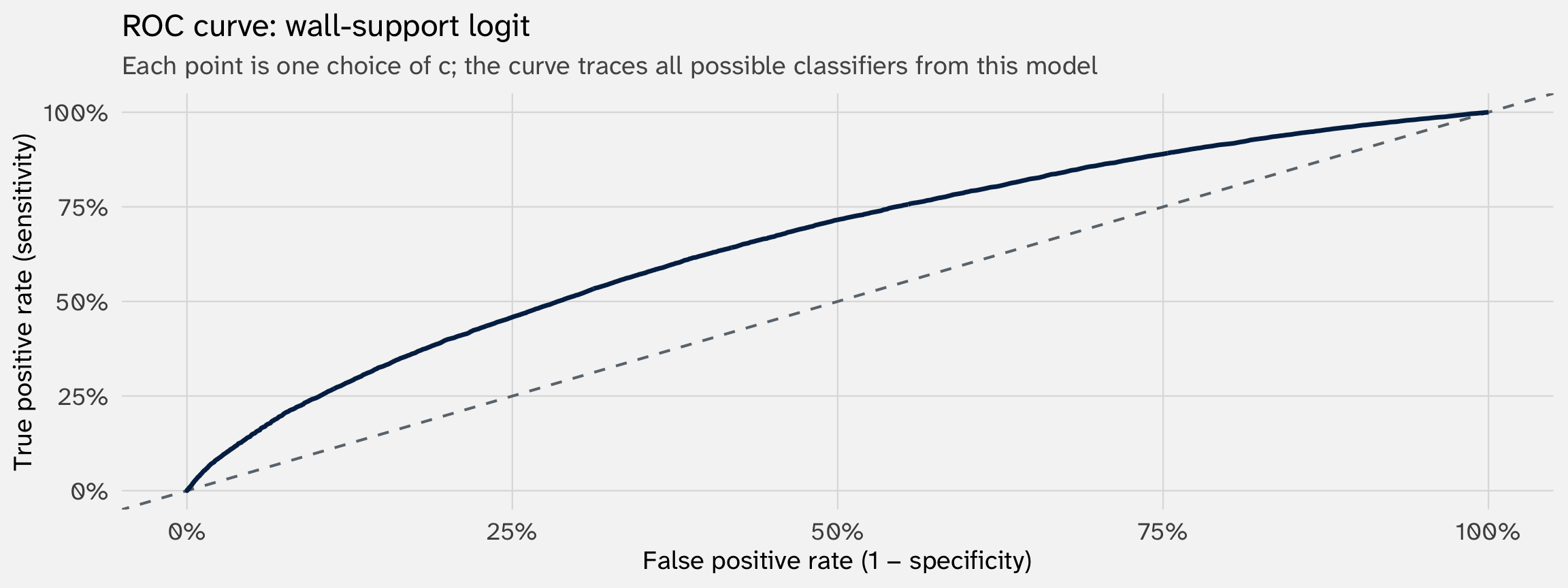
The dashed diagonal: a model that classifies by coin flip. TPR = FPR at every threshold
pROC::roc
pROC::roc() returns sensitivity (TPR) and specificity (1 - FPR)
AUC: the area under the curve
To summarize the curve in one number: AUC = area under the ROC curve, in \([0, 1]\).
Rules of thumb (these are made up):
- AUC = 0.5 → no better than chance
- 0.6–0.7 → meh-decent
- 0.7–0.8 → decent-good
- 0.8–0.9 → good-very good
- 0.9+ → excellent (and often suspicious)
Comparing models with AUC
What if we only knew a person’s age?
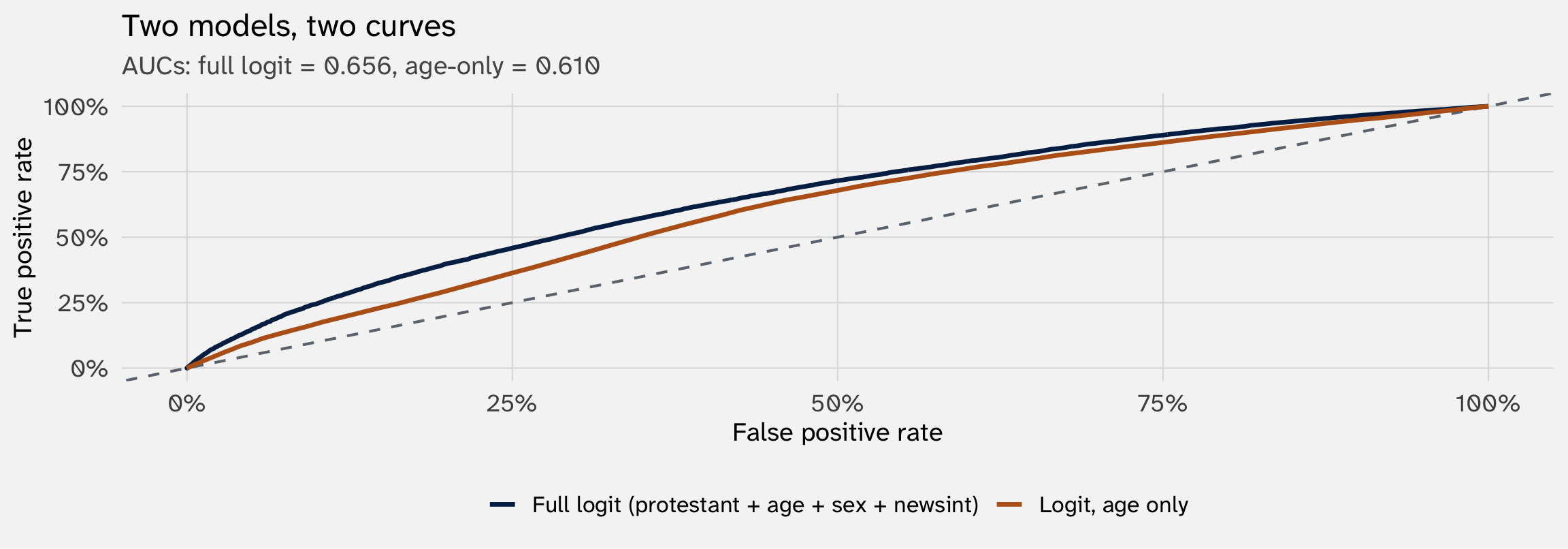
The gap between the two is the improvement in classification
What AUC does not tell you
One thing to notice first: AUC turns out to equal \(\Pr(\hat p_i > \hat p_j \mid y_i = 1, y_j = 0)\) — the probability a random supporter is ranked above a random opposer
1. AUC ignores magnitude. Two models that put observations in the same order but with very different spreads of \(\hat p\) — one \(\{0.49, 0.51\}\), the other \(\{0.01, 0.99\}\) — get the same AUC. The second is far more useful for actual decision-making, but AUC doesn’t see the difference
2. Class imbalance: AUC is robust to class imbalance (which is why it’s the default), but for very rare outcomes (e.g., 1% positives), precision-recall curves are often more informative
For many applications, AUC is the standard — but be aware it summarizes the model’s ordering of cases, not the quality of the predicted probabilities themselves
Your turn: predicting Obama voters
Use socviz::gss_sm (2016 GSS subset). Outcome: obama (1 = voted for Obama in 2012, 0 = voted for Romney). Fit a logit, evaluate its predictions
Steps:
- Fit a logit. Pick whatever predictors you want from
gss_sm
- Predict probabilities. Use
predict(mod, type = "response")to get a \(\hat p_i\) for each respondent
- Pick a threshold \(c\) of your choice. Build a confusion matrix with
table(actual = ..., predicted = as.integer(phat > c)). Compute TPR and FPR by hand from the table
- ROC curve and AUC. Use
pROC::roc()to compute the curve andpROC::auc()for the area. Plot the curve.
Summary so far
| Outcome type | Headline metric | What it measures |
|---|---|---|
| Continuous \(Y\) | MSE / \(R^2\) | Avg. squared distance / fraction of variance explained |
| Binary \(Y\) | AUC | Probability a random positive ranks above a random negative |
| Count \(Y\), ordered \(Y\), etc. | log-likelihood, deviance, pseudo-\(R^2\) | (Generalize the same idea; details vary) |
But there’s a big problem we’ve ignored. Every metric we just computed used the same data we fit the model on. This means:
- Our prediction metrics will tend to be too optimistic →
- In-sample prediction will mechanically improve as you add more explanatory variables / terms (e.g., polynomials) →
- So in-sample metrics can look strong even if the model is terrible at actual prediction (e.g., predicting the future / data that has not been observed yet)
2. In-sample lies; out-of-sample is more honest
An alien learns “vegetable”
An alien is on a research trip to Earth. They’ve never seen a vegetable. An Earthling shows them ten objects and tells them which is which. Call this the training set:
Vegetables
- 🥦 broccoli
- 🥕 carrot
- 🍅 tomato
- 🌶️ red pepper
- 🥬 lettuce
Not vegetables
- 🍎 apple
- 🐟 fish
- 🍰 cake
- 🪨 rock
- 🚗 car
Goal Write a model that classifies new objects as vegetables or not to use during grocery trip
Three rules, three accuracies
Model 1
“Vegetables are green”
On training set: broccoli + lettuce caught. But carrot, tomato, red pepper missed. Apple wrongly caught (some are green)
In-sample accuracy: ~50%
Verdict: too crude — misses the real pattern
Model 2
“Grows in dirt, eaten as part of a meal”
On training set: all five vegetables ✓, all five non-vegetables ✓
In-sample accuracy: ~100%
Verdict: captures the real pattern — onion, potato, mushroom (new objects) will likely also pass
Model 3
“Green OR orange OR red, smaller than a basketball, sold in grocery aisle 3–5, AND was on the table on Tuesday…”
On training set: all five vegetables ✓, all five non-vegetables ✓
In-sample accuracy: 100%
Verdict: memorized accidents — a brown potato fails, a vegetable in aisle 6 fails
The trap: models 2 and 3 both hit 100% on the training set. But on new objects — the ones you’ll actually see in the grocery store — model 2 wins, because model 3 only got to 100% by leaning on accidents (the aisle number) that won’t replicate
In-sample vs out-of-sample
In-sample: the data the model was fit on. The alien’s ten objects. The model has seen every observation and tuned the rule (or \(\hat\beta\)) to fit them as well as possible — by construction
Out-of-sample: data the model has never seen. The grocery store tomorrow. A more honest test of “would this work on a new sample?”
The lesson from the alien: a rule that fits the training data perfectly may have just memorized accidents — features that happened to be true of the training examples but don’t generalize (overfitting). The same is true of any model we estimate by minimizing in-sample loss: OLS, MLE, anything. In-sample fit improves with complexity by construction; out-of-sample fit is the more honest yardstick
You’ve been here before
In Week 2, we asked: if we fit a moderate and a flexible model to three independent random subsamples of the same data, do they tell the same story?
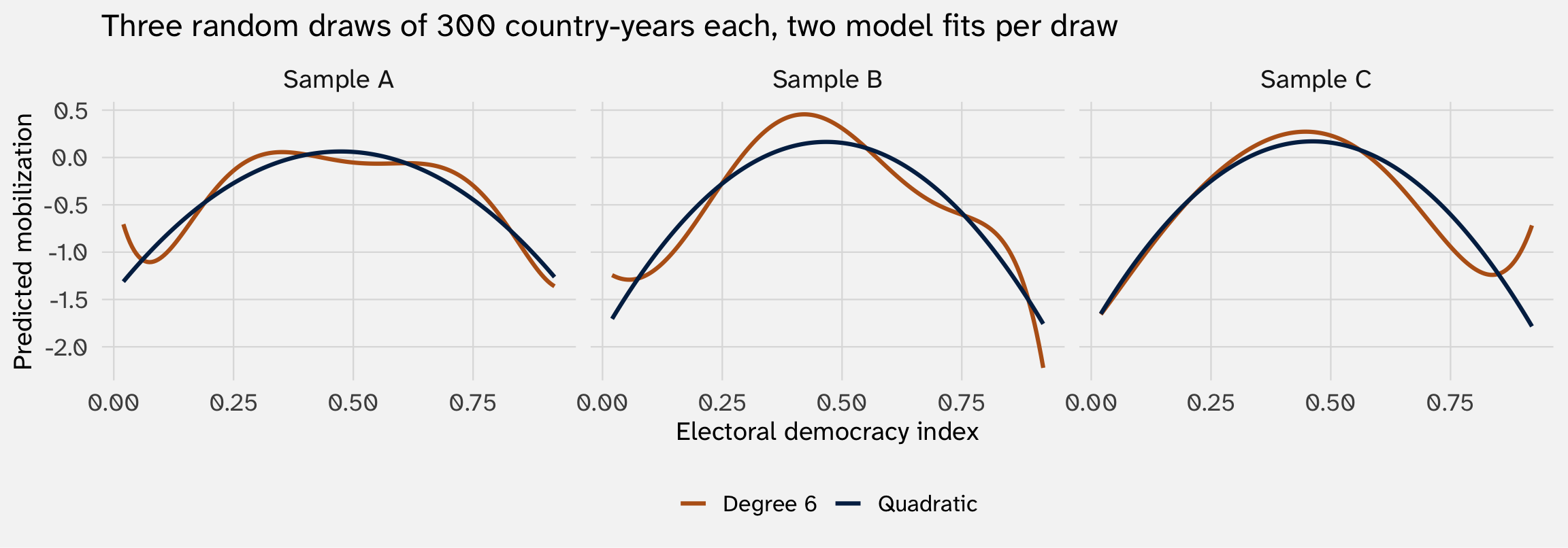
The quadratic tells the same story in all three samples. The degree-6 polynomial tells different stories — its wiggles are artifacts of which 300 country-years happened to land in each draw
A quick demonstration
Let’s exaggerate the difference: linear model, a quadratic, a degree-15 polynomial
set.seed(213)
protest_small = protest |> slice_sample(n = 300)

mods = list(
  lin  = lm(mobilization ~ democracy + ln_gdppc + ln_pop, data = protest_small),
  quad = lm(mobilization ~ poly(democracy, 2,  raw = TRUE) + ln_gdppc + ln_pop, data = protest_small),
  d15  = lm(mobilization ~ poly(democracy, 15, raw = TRUE) + ln_gdppc + ln_pop, data = protest_small)
)Each more flexible model has higher in-sample \(R^2\). Degree-15 wins on training fit. How will they do out-of-sample?
Where does out-of-sample data come from?
An intuitive approach is to compare a model based on present data to some future outcome (e.g., a weather forecast); some do this in the social sciences, but it’s rare
Common approach: fit your model to \(X\%\) of your data (training set); generate prediction metrics on remainder, \(100\%-X\%\) (test set)
n_train  n_test
    225      75
the {caret} package
The caret package was the gold standard for awhile; nowadays it seems like tidymodels
Compare in-sample to out-of-sample \(R^2\)
Refit each model on the training data only. Then compute \(R^2\) (or ROC, AUC, MSE, etc.) on the test data — observations the models have never seen
| model | r2_train | r2_test | gap |
|---|---|---|---|
| Linear | 0.088 | 0.056 | 0.032 |
| Quadratic | 0.165 | 0.155 | 0.010 |
| Degree 15 | 0.211 | 0.089 | 0.121 |
The story flips. In-sample, degree-15 looks best. Out-of-sample, quadratic wins
k-fold cross-validation
A single train/test split is noisy — what if you got an unlucky 25%? \(k\)-fold CV averages over many splits to reduce that noise:
- Randomly partition the data into \(k\) equal-sized folds (often \(k = 5\) or \(10\))
- For each fold \(j\): fit on the other \(k - 1\) folds, predict the held-out fold, compute the metric
- Average the \(k\) metrics
| Fold | Linear | Quadratic | Degree 15 |
|---|---|---|---|
| Fold 1 | 0.081 | -0.005 | 0.072 |
| Fold 2 | 0.019 | 0.067 | 0.089 |
| Fold 3 | 0.117 | 0.175 | 0.167 |
| Fold 4 | 0.139 | 0.280 | 0.246 |
| Fold 5 | 0.156 | 0.345 | 0.296 |
| Fold 6 | 0.055 | 0.216 | 0.254 |
| Fold 7 | 0.036 | 0.153 | 0.002 |
| Fold 8 | 0.118 | 0.174 | 0.162 |
| Fold 9 | 0.034 | 0.053 | -0.044 |
| Fold 10 | 0.072 | 0.191 | 0.127 |
| Mean | 0.083 | 0.165 | 0.137 |
The bias-variance tradeoff
The pattern: in-sample fit rewards complexity, out-of-sample fit doesn’t. Adding flexibility helps until it starts fitting noise — past that point, out-of-sample performance falls
This is the bias-variance tradeoff, the central organizing idea of machine learning. Simple models have high bias (they can’t fit the true signal well) but low variance (predictions are stable across resamples). Flexible models have low bias but high variance (their predictions are unstable, sample-to-sample)
Using OOS to evaluate variable importance
Many empirical papers define importance by statistical significance — \(X\) “matters” if \(p < 0.05\) (NHST). Long-standing critiques of this approach:
- Statistical significance \(\neq\) practical significance. Tiny, significant effect may not matter.
- With a large enough \(N\), significance easier to “find”
- \(p\)-values less well-defined in some political science applications (e.g., when you have “all” the data)
Ward, Greenhill & Bakke (2010) ask: does a significant variable actually increase a model’s predictive performance?
Notice the move here: the implication is that if a variable does not improve predictive performance, it does not help us understand \(Y\)
The Fearon-Laitin model
| Fearon-Laitin logit | |
|---|---|
| (Intercept) | −6.008*** |
| (0.762) | |
| log_pop | 0.218** |
| (0.078) | |
| log_gdp | −0.869*** |
| (0.139) | |
| polity2 | 0.042* |
| (0.017) | |
| mtnest | 0.006 |
| (0.005) | |
| oil | 1.026*** |
| (0.294) | |
| ef | −0.013 |
| (0.497) | |
| numlang | −0.000 |
| (0.016) | |
| Num.Obs. | 6124 |
| + p < 0.1, * p < 0.05, ** p < 0.01, *** p < 0.001 |
Significant at p < 0.05: log_pop, log_gdp, polity2, oil. Hold onto that list — we’ll ask which ones actually move OOS predictions
Build the model up, one variable at a time
What does each predictor add in out-of-sample AUC?
| Variable added | CV AUC | Δ AUC |
|---|---|---|
| intercept only | 0.5000 | NA |
| + log_gdp | 0.6943 | 0.1943 |
| + log_pop | 0.6918 | -0.0025 |
| + polity2 | 0.7163 | 0.0245 |
| + oil | 0.7261 | 0.0098 |
| + ef | 0.7209 | -0.0052 |
| + numlang | 0.7208 | -0.0001 |
| + mtnest | 0.7211 | 0.0003 |
Significane and prediction: log_pop is statistically significant at p < 0.01 in the full model — but adding it to a model that already has log_gdp decreases CV-AUC by -0.0025. The coefficient is reliably non-zero; the variable is just not predictively useful (given the other predictors)
What this means
Statistical significance answers: “is this coefficient reliably non-zero in repeated samples?” Useful for interpretation
Predictive value answers: “if I know this variable, do I predict \(Y\) better than without it?” Useful for prediction — when you want to use the model to forecast new observations
They can disagree: a variable can be highly significant but predictively trivial (large sample → tiny effects look “significant”); a variable can be predictively powerful but not statistically significant in a tiny sample. Big-N political-science data has lots of the first case
The Statisticians’ view on good inferences
With these metrics for evaluating how well a model predicts, the Statistician(™) says the following:
- “Model X has poor predictive performance; it is unlikely to be reproducing the DGP; we should not take inferences drawn from it seriously”
- “Model Y has good predictive performance; it is likely to be reproducing the DGP; we should take inferences drawn from it (more) seriously”
These are all ways of evaluating the quality of research → \(\widehat{Y}\)
So far: linear-in-parameters models \(\beta X\) → we pick predictors (age, race, sex, etc) and functional form (quadratic, not quadratic, etc.) that are still interpretable
What if we instead use algorithms to pick predictors and functional form?
Your turn: out-of-sample prediction
Go back to the previous activity’s model/data predicting support for obama.
Steps:
Fit a logit, excluding one region. Exclude one region (
bigregion) from your model.Generate in-sample and OOS predictions. Generate predictions for the three regions in your training data and the one region in your test data.
ROC curve and AUC. Use
pROC::roc()pROC::auc()for the area.Repeat for all regions. Cycle through the other regions, treating each as out-of-sample. Which region is hardest to predict?
3a. Beyond linear-in-parameters
Let \(\hat y = f(X)\) for whatever \(f\) the data want
The big shift
Everything before this slide assumed:
\[\hat y_i \;=\; g(X_i\beta)\]
for some known link function \(g\) (identity for OLS, \(\sigma\) for logit, \(\exp\) for Poisson). The structure of the relationship — which is linear in \(\beta\), and additive in covariates — was chosen by us
Machine learning models say: pick a function class flexible enough to capture any relationship, then let the algorithm find which function in that class fits best.
\[\hat y_i \;=\; f(X_i) \quad \text{for } f \text{ from a very flexible family}\]
Different ML algorithms = different function families. We’ll climb the ladder
Rung 1 — GAM (additive but smooth)
Generalized additive models keep the additivity of the linear model but let each predictor’s contribution be a smooth nonlinear function:
\[\hat y_i \;=\; \beta_0 \;+\; f_1(x_{i1}) \;+\; f_2(x_{i2}) \;+\; \ldots \;+\; f_k(x_{ik})\]
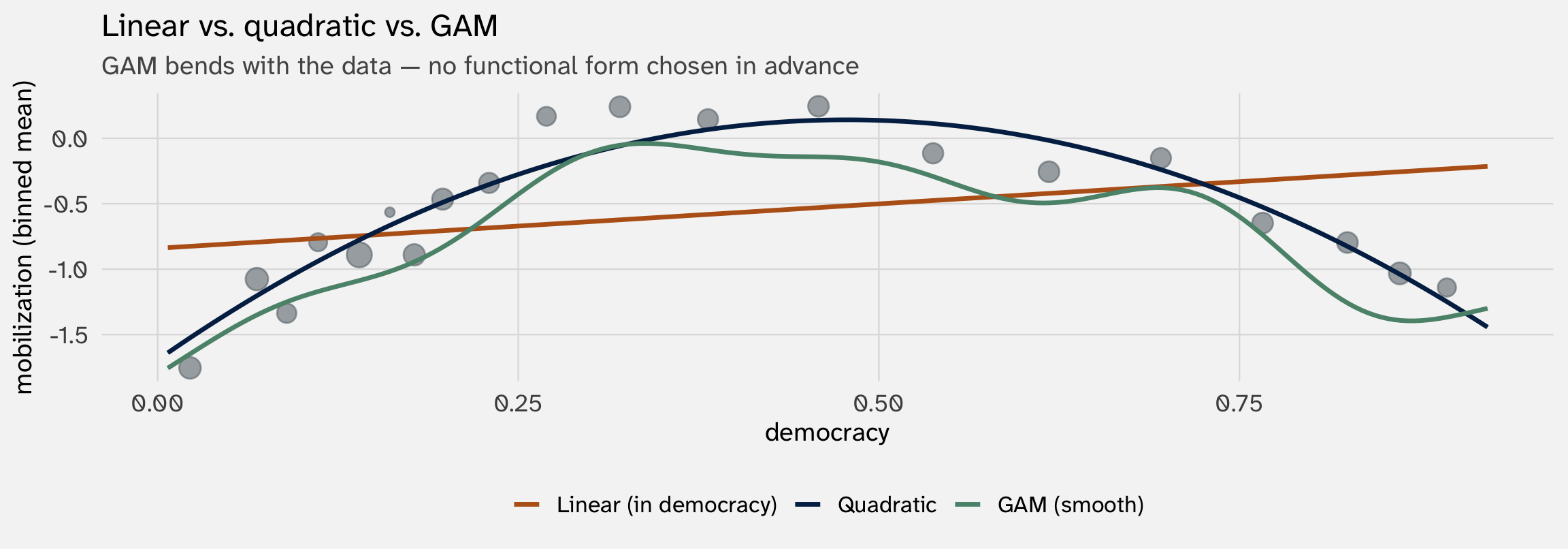
You can still plot each \(f_k\) — interpretability mostly survives. GAMs are a gentle step away from OLS
Rung 2 — KNN (no model, just neighbors)
K-nearest neighbors: for each new observation, find the \(k\) closest training points and average their \(y\) values
\[\hat y_i \;=\; \frac{1}{k} \sum_{j \in N_k(X_i)} y_j\]
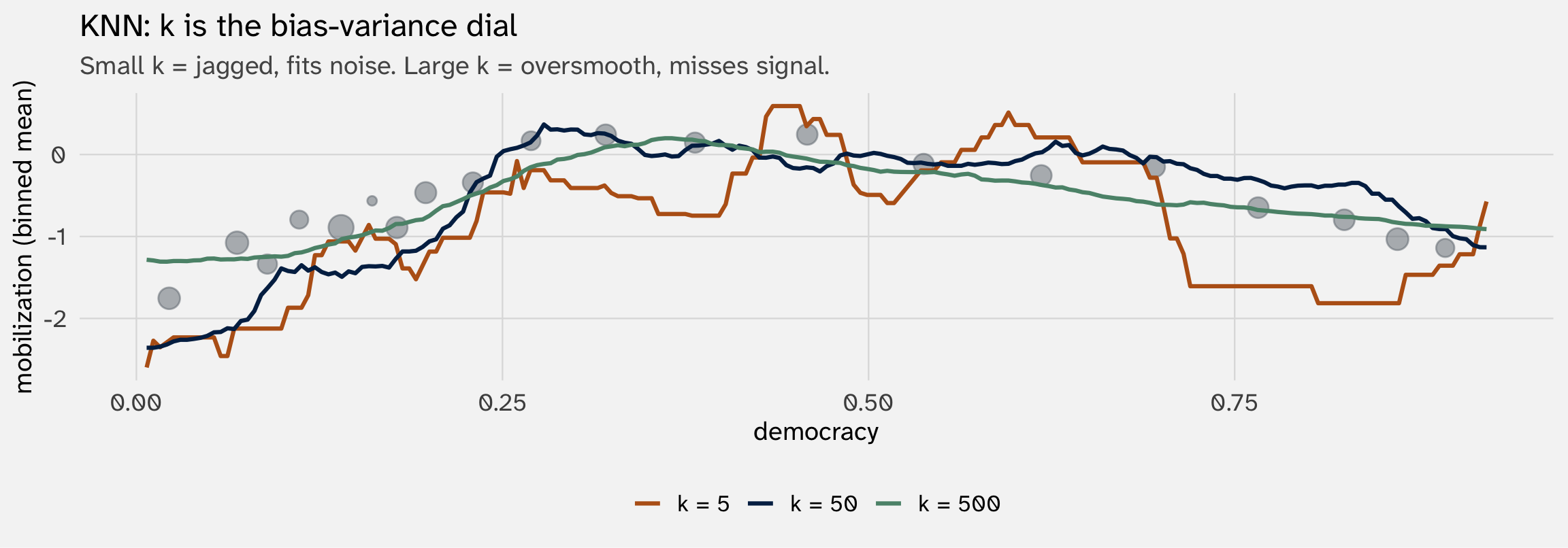
What’s new: no parameters, no model, no \(\hat\beta\). You just decide how close or far away to look for each observation
Rung 3 — Decision trees and random forests
Create a “flowchart” of conditional rules based on \(X\). Pick rules that most improves classification / reduces error. Each “leaf” is a prediction (mean of \(y\) for observations that land there)
Protestant?
├── no  (Non-Protestant, n = 41,601) → age ≥ 42.5?
│   ├── no:  ŷ = 0.25   (younger non-Protestants → low support)
│   └── yes: ŷ = 0.40
└── yes (Protestant,     n = 19,265) → sex == Male?
    ├── no:  ŷ = 0.46
    └── yes: ŷ = 0.63   (Protestant men → highest support)
A single tree is readable — But it’s high-variance: tiny changes to the data can produce completely different results. To stabilize, we average across many, producing random forest
Why random forest works: each tree is high-variance, but the errors don’t all line up — averaging cancels them out. The forest has much lower variance than any single tree, at the cost of losing the flowchart-interpretation
Rung 4 — Gradient boosting
Sequentially fit shallow trees, each one correcting the previous tree’s errors. Combine them additively:
\[\hat y \;=\; \sum_t \eta \cdot \hat f_t(X) \quad \text{where each } \hat f_t \text{ fits the residuals from } \hat f_{t-1}\]
The current-ish “state of the art” for tabular data: xgboost, lightgbm, catboost. Hyperparameter tuning is more involved than random forests, but performance ceiling is higher
Same tradeoffs as RF, more so: high accuracy, low interpretability, requires careful cross-validation
Rung 5 — Neural networks (briefly)
Hierarchical compositions of linear transformations + nonlinear activations:
\[\hat y \;=\; g_L\!\big( W_L \cdots g_2(W_2 \cdot g_1(W_1 X)) \big)\]
Dominant for unstructured data — images, text, audio. For tabular political-science data, they usually lose to gradient boosting. They shine when the data has a structure ML models can exploit (pixel grids, word sequences)
For the kinds of datasets you’ll work with in PS dissertations, neural nets are rarely the right tool unless you’re doing text-as-data or image work
Bake-off: logit vs. xgboost on wall
How do logit and gradient boosting compare at predicting who supports the wall (wall = 1)?
🥁🥁🥁🥁🥁🥁
| model | cv_auc |
|---|---|
| Logit | 0.656 |
| Gradient boosting (xgboost) | 0.661 |
Sad! But also:
- machine learning models benefit from tuning of hyperparameters, which we didn’t do here
- machine learning as an approach does not care about specific parameters → you might cycle through many
BUT ALSO:
- at least for tabular data, more flexible models are not necessarily better at prediction
What did we win? What did we lose?
Gradient boosting’s CV-AUC is slightly higher than the logit’s. With these few predictors and a fairly linear problem, the gap is modest
Now ask: What do we lose?
There is no coefficient table. The model is mostly a black box. No \(\hat\beta_{\text{protestant}}\) exists to report. You can’t say “controlling for age, sex, and news interest, being Protestant is associated with a 20-percentage-point increase in predicted wall support.” That sentence requires linear-in-parameters
This is the interpretability tax of leaving the linear-in-parameters scaffold; another tradeoff: more flexible models are less interpretable
There are a few machine learning approaches to recover some interpretability
3b. The interpretability tradeoff
Three partial recoveries of \(\hat\beta\)
What \(\hat\beta\) gave us, for free
In every MLE model in this course, each \(\hat\beta_k\) gave us:
- Direction — sign of the effect (does \(X_k\) push \(Y\) up or down?)
- Magnitude — size of the effect (how much per unit?)
- Uncertainty — standard error, \(p\)-value, CI
- A clean sentence — “a one-unit increase in \(X_k\) is associated with…”
Random forests, boosting, neural nets give you none of these directly. We have to reconstruct them with auxiliary tools — each of which recovers a piece of what \(\hat\beta_k\) gave for free
Tool 1 — Variable importance
For each predictor, how much does predictive accuracy degrade if you randomly permute that predictor’s values? Big drop → important predictor
       age protestant        sex    newsint
    0.0150     0.0148     0.0061     0.0040
What you get: a ranking. Which features matter most
What you don’t get: direction (positive or negative?), magnitude on the outcome scale, uncertainty
Tool 2 — Partial dependence plots (PDPs)
For predictor \(X_k\), plot the model’s average prediction across the data, varying only \(X_k\):
\[\widehat{\text{PD}}_k(x) \;=\; \frac{1}{n} \sum_{i=1}^n \hat f\!\left(x, X_{i, -k}\right)\]
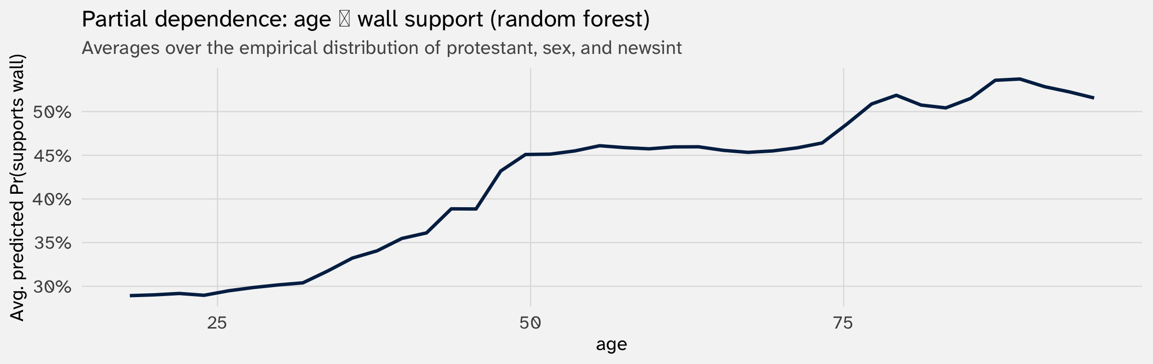
Recovers direction + a magnitude-like curve — but hides interactions and averages over correlated predictors
Each is a partial recovery
| What \(\hat\beta_k\) gives | Partial-recovery tool |
|---|---|
| Direction | PDP |
| Magnitude (output scale) | PDP |
| Magnitude (input scale, ranking) | Variable importance |
| Uncertainty | (Often missing; bootstrap can help) |
| One-sentence summary | Hard |
None of these are as clean as \(\hat\beta_k\). They each reclaim a piece of what the coefficient gave us, with caveats
That’s the tax we pay for flexibility. Whether it’s worth paying depends on your goal
Linear-in-parameters was a choice
The whole MLE curriculum is built on linear-in-parameters: \(X\beta\) sits inside the link function, and that gives us one readable \(\hat\beta_k\) per covariate. We did not have to do it this way. We chose to
Why? Because political science is mostly an explanatory discipline:
- “What effect does X have on Y?”
- “Which mechanism dominates?”
- “Does this theory’s prediction line up with the data?”
All of these require interpretation, not just prediction. They require us to read the model. Linear-in-parameters keeps the model readable
When ML is the right tool: when prediction is the goal — election forecasting, conflict early-warning systems, scoring applications. Then the interpretability tax is a price worth paying