| age | sex | degree | race | T_prog | Y |
|---|---|---|---|---|---|
| 47 | Male | Bachelor | White | 0 | 1.4 |
| 61 | Male | High School | White | 0 | -0.8 |
| 72 | Male | Bachelor | White | 0 | 2.5 |
| 43 | Female | High School | White | 0 | -1.8 |
| 55 | Female | Graduate | White | 0 | 2.8 |
| 53 | Female | Junior College | White | 0 | -1.1 |
Causal Inference with MLE & ML
POL 213 · Week 9
Juan F. Tellez
University of California, Davis
May 27, 2026
Housekeeping
- Final exam Wednesday June 3 (in class, closed book)
- Final paper due June 8
Two paths
The other one now
Which way?
(recap from last week)
The economist
Identify a treatment effect — get \(\hat\beta\) right.
- Key question: what’s the effect of \(X\) on \(Y\)?
- Worry list: confounding, selection, identification
- Holds \(\hat\beta\) to a high standard; doesn’t much care about \(\hat y\)
The statistician
Model the data-generating process — get \(\hat y\) right.
- Key question: how well do we predict \(Y\) from \(X\)?
- Worry list: predictive performance, overfitting
- Holds \(\hat y\) to a high standard; doesn’t much care about any particular \(\hat\beta\)
Last week we walked the statistician’s path → prediction & ML. This week we look at what MLE and ML have to say about causal inference
To walk the Economist Path™ you should take causal inference
Today’s plan
Two areas where prediction and ML are being used in causal inference:
- How can we deal with confounding? — Tools we’ll cover: propensity-score matching and related balancing methods.
- How much do treatment effects vary across subgroups? — Estimate heterogeneous treatment effects (HTE). Tool: causal forests (Athey & Wager).
Throughout: both of these problems lean on MLE models you already know (logit, OLS) and ML models from last week (random forests)
1. The causal inference problem
Can we do anything about confounding?
A running example: simulated workforce training
We’ll simulate data for a “JobTrain 2024” program that offers free job-training to American adults. We’d like to know what effect this program has on a standardized earnings index (Y)
Why simulate? Because the only way to check whether a causal method works is to know the truth. Here, we know:
- Enrollment in the program is voluntary. Relative to non-participants, participants tend to be younger, less-educated, slightly-more-female
- True effect (ATE) = +0.5 (every enrollee gets a 0.5-SD earnings boost)
- The participation variables (
age,degree,sex) also predict Y → older respondents earn more, education earns more, women earn less
The simulated data
| T_prog | n | share |
|---|---|---|
| 0 | 2302 | 80.8% |
| 1 | 547 | 19.2% |
About 19% of respondents enroll in the program. That’s our treated group
The naive estimate: just regress Y on T
The simplest possible “effect” estimate: regress earnings on the treatment indicator
| Naive: Y ~ T | |
|---|---|
| (Intercept) | −0.360*** |
| (0.032) | |
| T_prog | −0.725*** |
| (0.074) | |
| Num.Obs. | 2849 |
| R2 | 0.033 |
| + p < 0.1, * p < 0.05, ** p < 0.01, *** p < 0.001 |
The naive estimate is very wrong. The naive estimate says the program decreases earnings by about 0.7 SD — with a tiny SE and \(p < 10^{-20}\). The 95% CI doesn’t include zero, doesn’t include the true +0.5
But we set the true ATE to +0.5 (positive). What happened?
Why the naive comparison fails: confounding
The treated and control groups aren’t comparable:
| Treated? | n | Mean age | % female | Mean degree (1–5) |
|---|---|---|---|---|
| 0 | 2302 | 51.20 | 0.52 | 2.81 |
| 1 | 547 | 40.49 | 0.69 | 2.06 |
The treated are systematically younger, more female, and less educated (our design)
All three of those features also depress baseline earnings (our design)
So even though the program adds +0.5 to everyone, the treated start from a much lower baseline — and the naive comparison absorbs all of that selection into the “effect”
The approach
The problem: treatment wasn’t randomly assigned. The treated and control groups are too dissimilar to compare directly.
The hope: what if we could find a subset of respondents who do look very similar on age, education, sex — but where some got the program and some didn’t? Within that subset, treatment is closer to random.
One approach: matching respondents on their propensity to receive treatment
2. Balance and propensity scores
Diagnosing imbalance
First, we can see where the imbalance lies:
cobalt::bal.tab() gives us the standardized mean difference (SMD) between treated and control
What we knew by design: age, female, deg_num are the problem
A visual: love plot
Reading it: each dot is one covariate’s standardized mean difference. The dashed lines at ±0.1 mark “acceptable” (rule of thumb)
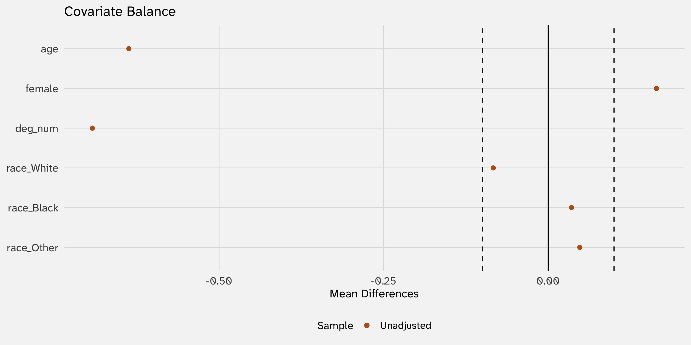
Ideally: we would pick a subset of respondents who are of similar ages, sex, education (without worsening balance on other variables)
How can we match on lots of variables at once?
In theory, go through every treated person, and look for an identical (or very similar) person who did not receive the program (control)
# A tibble: 5 × 6
      Y T_prog   age sex    degree         race
  <dbl>  <int> <dbl> <fct>  <fct>          <fct>
1 -2.08      1    23 Female High School    Other
2 -1.27      1    33 Female High School    White
3 -2.47      1    62 Female Lt High School Other
4 -1.07      1    43 Male   High School    Black
5 -2.77      1    32 Female Lt High School Black
# A tibble: 5 × 6
Y T_prog age sex degree race
<dbl> <int> <dbl> <fct> <fct> <fct>
1 1.38 0 47 Male Bachelor White
2 -0.786 0 61 Male High School White
3 2.50 0 72 Male Bachelor White
4 -1.76 0 43 Female High School White
5 2.80 0 55 Female Graduate WhiteIn most cases this is impossible. With 5 degree levels × 2 sexes × 70 age values, that’s 700 cells — many will be empty, even with 2,800 respondents. Curse of dimensionality
Rosenbaum & Rubin’s insight (1983): collapse the whole high-dimensional \(X\) into a single number — the propensity score:
\[\pi(X) \;=\; \Pr(T = 1 \mid X)\]
Estimating propensity scores with a logit
A propensity score is just a probability — model it with a logit:
| (1) | |
|---|---|
| + p < 0.1, * p < 0.05, ** p < 0.01, *** p < 0.001 | |
| (Intercept) | 1.549*** |
| (0.213) | |
| age | -0.040*** |
| (0.003) | |
| female | 0.881*** |
| (0.109) | |
| deg_num | -0.706*** |
| (0.057) | |
| raceBlack | -0.036 |
| (0.134) | |
| raceOther | 0.145 |
| (0.164) | |
The recipe: regress \(T\) on all the covariates you think determine who receives treatment
Propensity scores
The fitted probabilities \(\hat\pi_i = \widehat{\Pr}(T_i = 1 \mid X_i)\) are the propensity scores
# A tibble: 2,849 × 42
   pscore  year    id ballot       age childs sibs     degree race  sex   region
    <dbl> <dbl> <dbl> <labelled> <dbl>  <dbl> <labell> <fct>  <fct> <fct> <fct>
 1 0.0404  2016     1 1             47      3 2        Bache… White Male  New E…
 2 0.0896  2016     2 2             61      0 3        High … White Male  New E…
 3 0.0152  2016     3 3             72      2 3        Bache… White Male  New E…
 4 0.329   2016     4 1             43      4 3        High … White Fema… New E…
 5 0.0351  2016     5 3             55      2 2        Gradu… White Fema… New E…
 6 0.139   2016     6 2             53      2 2        Junio… White Fema… New E…
 7 0.133   2016     7 1             50      2 2        High … White Male  New E…
 8 0.559   2016     8 3             23      3 6        High … Other Fema… Middl…
 9 0.153   2016     9 1             45      3 5        High … Black Male  Middl…
10 0.0315  2016    10 3             71      4 1        Junio… White Male  Middl…
# ℹ 2,839 more rows
# ℹ 31 more variables: income16 <fct>, relig <fct>, marital <fct>, padeg <fct>,
#   madeg <fct>, partyid <fct>, polviews <fct>, happy <fct>, partners <fct>,
#   grass <fct>, zodiac <fct>, pres12 <labelled>, wtssall <dbl>,
#   income_rc <fct>, agegrp <fct>, ageq <fct>, siblings <fct>, kids <fct>,
#   religion <fct>, bigregion <fct>, partners_rc <fct>, obama <dbl>,
#   deg_num <dbl>, female <int>, eta_T <dbl>, p_T <dbl>, T_prog <int>, …
Distribution of propensity scores
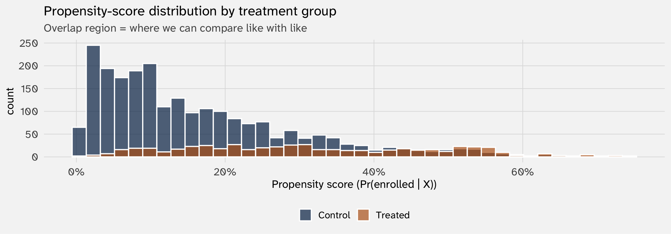
Two things to look for:
- Imbalance: are the two distributions in very different places? Big imbalance → big selection problem. Small imbalance → the data are already nearly balanced
- Overlap (common support): is there a region where both groups have observations? These are observations that are comparable → similar propensity to treatment, but different treatment statuses
3. Propensity-score matching
Pair each treated case with a similar control
The idea
For each treated observation \(i\), find the control observation \(j\) with the closest propensity score \(\hat\pi_j \approx \hat\pi_i\). Compare \(Y_i\) to \(Y_j\) within the pair. Average across pairs
| Pair | Role | Age | Sex | Degree | π | | |
|---|---|---|---|---|---|---|
| 1 | Treated | 36 | Female | Bachelor | 0.13 | 1.29 |
| 1 | Control | 36 | Female | Bachelor | 0.13 | 0.77 |
| 2 | Treated | 51 | Female | High School | 0.26 | -1.31 |
| 2 | Control | 51 | Female | High School | 0.26 | -1.43 |
| 3 | Treated | 33 | Male | Lt High School | 0.42 | -2.67 |
| 3 | Control | 33 | Female | High School | 0.41 | -2.37 |
| 4 | Treated | 21 | Female | High School | 0.58 | -1.83 |
| 4 | Control | 21 | Female | High School | 0.58 | -2.49 |
Read it: within each pair, the propensity scores are essentially identical. Their \(Y\) values differ, and the average of those within-pair differences is our matched ATE estimate
Why this should work: if two people were truly equally likely to receive treatment, but only one did for random/idiosyncratic reasons, then they are exchangeable
Matching with MatchIt
Call:
matchit(formula = T_prog ~ age + female + deg_num + race, data = gss_train,
    method = "nearest", distance = "glm", ratio = 1)

Summary of Balance for All Data:
          Means Treated Means Control Std. Mean Diff. Var. Ratio eCDF Mean
distance         0.3183        0.1620          0.9234     1.5519    0.2536
age             40.4936       51.2020         -0.6617     0.8640    0.1487
female           0.6874        0.5230          0.3546          .    0.1644
deg_num          2.0622        2.8128         -0.8382     0.5180    0.1501
raceWhite        0.6654        0.7489         -0.1769          .    0.0835
raceBlack        0.1993        0.1638          0.0889          .    0.0355
raceOther        0.1353        0.0873          0.1402          .    0.0480
          eCDF Max
distance    0.4096
age         0.2686
female      0.1644
deg_num     0.2527
raceWhite   0.0835
raceBlack   0.0355
raceOther   0.0480

Summary of Balance for Matched Data:
          Means Treated Means Control Std. Mean Diff. Var. Ratio eCDF Mean
distance         0.3183        0.3090          0.0548     1.1236    0.0050
age             40.4936       41.3729         -0.0543     1.0101    0.0128
female           0.6874        0.7221         -0.0749          .    0.0347
deg_num          2.0622        2.1042         -0.0470     1.1431    0.0157
raceWhite        0.6654        0.6600          0.0116          .    0.0055
raceBlack        0.1993        0.2230         -0.0595          .    0.0238
raceOther        0.1353        0.1170          0.0535          .    0.0183
          eCDF Max Std. Pair Dist.
distance    0.0585          0.0558
age         0.0420          0.3935
female      0.0347          0.2879
deg_num     0.0603          0.3246
raceWhite   0.0055          0.5541
raceBlack   0.0238          0.5355
raceOther   0.0183          0.5452

Sample Sizes:
          Control Treated
All          2302     547
Matched       547     547
Unmatched    1755       0
Discarded       0       0
What MatchIt does:
- Fits a propensity-score logit (same as above)
- For each treated unit, finds the nearest-propensity control
- Returns a “matched” dataset where each treated unit has one paired control
Did matching balance the covariates?
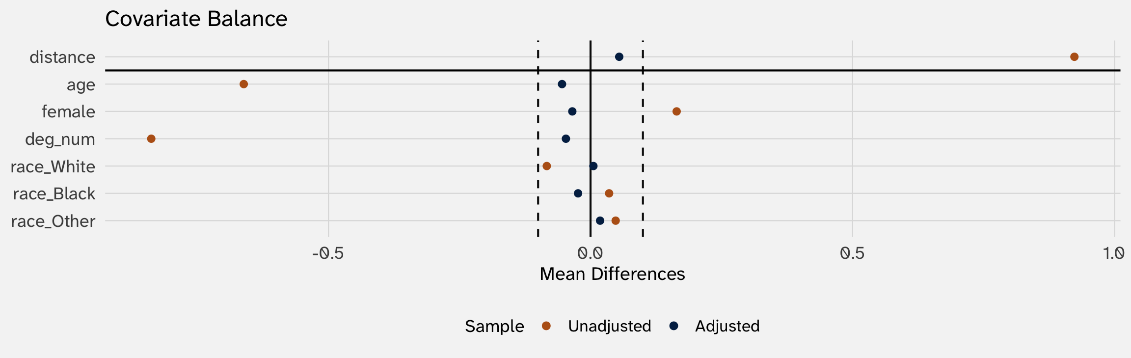
Read the plot: each variable has two dots — one for the original (unadjusted) sample, one after matching. Matching should pull all the post-match dots inside the ±0.1 band
Estimating the ATE from matched data
| Naive (full sample) | PSM (matched sample) | |
|---|---|---|
| (Intercept) | −0.360*** | −1.541*** |
| (0.032) | (0.052) | |
| T_prog | −0.725*** | 0.456*** |
| (0.074) | (0.074) | |
| Num.Obs. | 2849 | 1094 |
| R2 | 0.033 | 0.034 |
| + p < 0.1, * p < 0.05, ** p < 0.01, *** p < 0.001 |
Truth: \(\tau = +0.5\). Naive is wildly off; matching pulls us back to a positive estimate within sampling noise of the true effect
How is this different from just controlling for X?
We’ve used lm(Y ~ T + X) to “control for \(X\)” plenty of times. What does matching do that’s different?
Controlling for \(X\) (lm(Y ~ T + X))
- Adjusts for \(X\) inside the model
- Imposes a functional form (usually linear, additive) on \(X \to Y\)
- Uses all observations — silently extrapolates to regions where you have no overlap
- Adjustment is invisible: one \(\hat\beta_T\) comes out the other side
Matching on \(X\)
- Adjusts for \(X\) before the model
- No functional form assumption between \(X\) and \(Y\)
- Observations without similar matches get dropped — lack of overlap is visible
- Adjustment is auditable: love plot + balance table tell you whether it worked
Matching is not magic just as with “control for \(X\)”, if you miss an \(X\), mis-measure it, etc., the estimate will be biased
Use ML to predict treatment
Last week, we saw that the trade-off with ML was better predictions but terrible interpretability (because we drop linear-in-parameters)
But the propensity model is a place where we don’t care — we’re mostly not going to interpret coefficients on the propensity logit. We just want good predictions of treatment (\(\pi\))
That makes it a natural home for ML. Swap the propensity model from logit to random forest with one argument:
When is ML clearly better?: ML propensity scoring isn’t automatically better. It’s better when the true selection mechanism is nonlinear or interactive. The choice is empirical: pick whichever produces a cleaner-looking matched sample
Beyond propensity scores
King & Nielsen (2019): “Why propensity scores should not be used for matching” (Political Analysis)
Propensity scores are just one way of defining similarity; arguably, there are better ways
Other matching methods measure similarity differently:
- Coarsened exact matching (CEM) — bin each covariate (e.g., age in 10-year buckets), then require treated/control pairs to share the same cell
- Genetic matching — search over weights on covariates to find a distance metric that optimizes balance
- Entropy balancing — directly reweight controls so the weighted control distribution matches the treated distribution on specified moments
The big picture: These are all methods for finding similar observations. They differ in how they measure similarity (a scalar score, a cell, a weighted distance, distributional moments). Same goal, different tools
The recipe so far
Five-step PSM workflow:
- Decide which \(X\) confounds \(T \to Y\). (Theory, DAGs, common sense)
- Pick a similarity metric: propensity score (logit / RF / xgboost), exact-on-bins (CEM), distance-on-weighted-covariates (genetic), or moment-matching (entropy balancing)
- Diagnose balance:
cobalt::bal.tabandlove.plot. Iterate on the metric or specification if balance is bad - Match (or weight, or stratify): pair / reweight units that are similar on the chosen metric
- Estimate the effect on the balanced sample: regression of \(Y\) on \(T\) (with or without additional covariate adjustment)
Matching isn’t magic (don’t forget!):
- Everything hinges on conditional unconfoundedness — if you missed a confounder, the estimate is still biased
Your turn: matching on juanr::affairs
Use juanr::affairs. Outcome n_affairs (count of extramarital affairs reported). “Treatment”: kids (1 = has children, 0 = doesn’t)
- Pre-match balance:
cobalt::bal.tab(kids ~ ..., data = affairs). Where are treated and control most imbalanced?
- Match:
matchit(kids ~ ..., data = affairs, method = "nearest", distance = "glm").
- Post-match balance: love plot on the matched object. Did matching close the gaps?
- Treatment effect: extract the matched sample with
match.data()and fitlm(n_affairs ~ kids, data = matched). Compare to the naive estimate (no matching). Interpret
4. Heterogeneous treatment effects
Beyond the average — who does the program help most?
Average treatment effects are just the average
Most of the time you are struggling to estimate the ATE — the average treatment effect across the whole sample. But any treatment could affect people very differently depending on who they are
- Maybe a jobs program helps younger workers a lot and older workers little
- Maybe being a victim makes some people trust the state more and others less
- Maybe exposure to pollution hurts some communities more than others
Why we care: if a program helps some subgroups and hurts others, “expand it” and “kill it” introduces tradeoffs
A working example: peer judgments in Taiwan
Working paper with coauthors (N ≈ 3,000 Taiwanese respondents). The experiment:
- Respondents engage in a moral decision-making game — assigning blame to people who did bad things in the past
- Randomly assigned: a peer-influence prime that purports to show “how prior respondents like you behaved”
- Outcome: their own blame attributions
The main finding: exposure to the peer prime shifts blame attribution by about +11 percentage points in the direction of the displayed peers. That’s the average treatment effect among all respondents
The new question: in theory, this effect should vary across people. Some are more susceptible to peer pressure than others. Who is the peer effect strongest among?
The standard approach: interact treatment with a moderator
Suppose theory says news consumers might be more (or less) susceptible. Fit:
\[Y_i \;=\; \beta_0 \;+\; \beta_1 T_i \;+\; \beta_2 \text{NewsHigh}_i \;+\; \beta_3 (T_i \times \text{NewsHigh}_i) \;+\; \varepsilon_i\]
| Term | Estimate | Std. Error |
|---|---|---|
| (Intercept) | 0.211** | (0.014) |
| Peer prime (T) | 0.080** | (0.020) |
| News consumer = High | -0.022 | (0.018) |
| T × News consumer = High | 0.062* | (0.028) |
Reading the table: peer effect for low news consumers \(= \hat\beta_1 \approx 0.08\). For high news consumers \(= \hat\beta_1 + \hat\beta_3 \approx 0.14\). News consumers appear more responsive — almost twice the effect
The challenge: too many moderators
This works when we have one moderator we care about. But:
With many possible moderators (\(X_1, X_2, \ldots, X_p\)) — age, political knowledge, partisanship, education, need-for-closure, religiosity, region — and possible interactions among them, hand-coding a regression with the “right” interactions becomes a fishing expedition
Three problems:
- We’ll always find some significant interaction by chance (\(p < 0.05\) on 20 tests \(\Rightarrow\) one false positive expected)
- We have to pre-specify which interactions to test, and theory rarely picks them out cleanly
- Three-way interactions (\(T \times X_1 \times X_2\)) are nearly impossible to interpret
We need a way to let the data tell us where the heterogeneity lives — without fishing
Causal forests (Athey & Wager 2019)
The idea: extend last week’s random forest, but each tree is built to predict the treatment effect at \(X = x\) rather than the outcome \(Y\)
For each observation \(i\), the forest returns an estimated individual treatment effect:
\[\hat\tau(X_i) \;=\; \text{forest's best estimate of } \;E[Y(1) - Y(0) \mid X = X_i]\]
Why this does what we want:
- no pre-specification we don’t choose which interactions to test. The forest searches the covariate space automatically
- guards against spurious discovery via principled sample splitting — training data used to fit heterogenous effects, testing data
- regularization of treatment effects meaning that detected heterogeneous effects must be consistent across a large number of subsamples to be considered meaningful
Distribution of estimated peer effects
Causal forest returns individual peer effects (based on covariates)
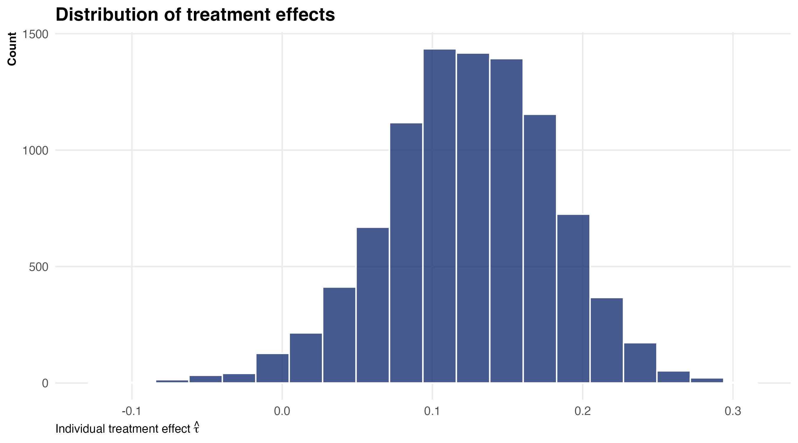
Effects are mostly positive (bulk between 0 and 0.3 — peer judgments shift blame attributions for almost everyone) but with real spread (from about \(-0.05\) to \(+0.30\))
Which variables drive the heterogeneity?
Causal forest can calculate variable importance (i.e., if you drop a variable, how much does it hurt the models’ predictive performance?)
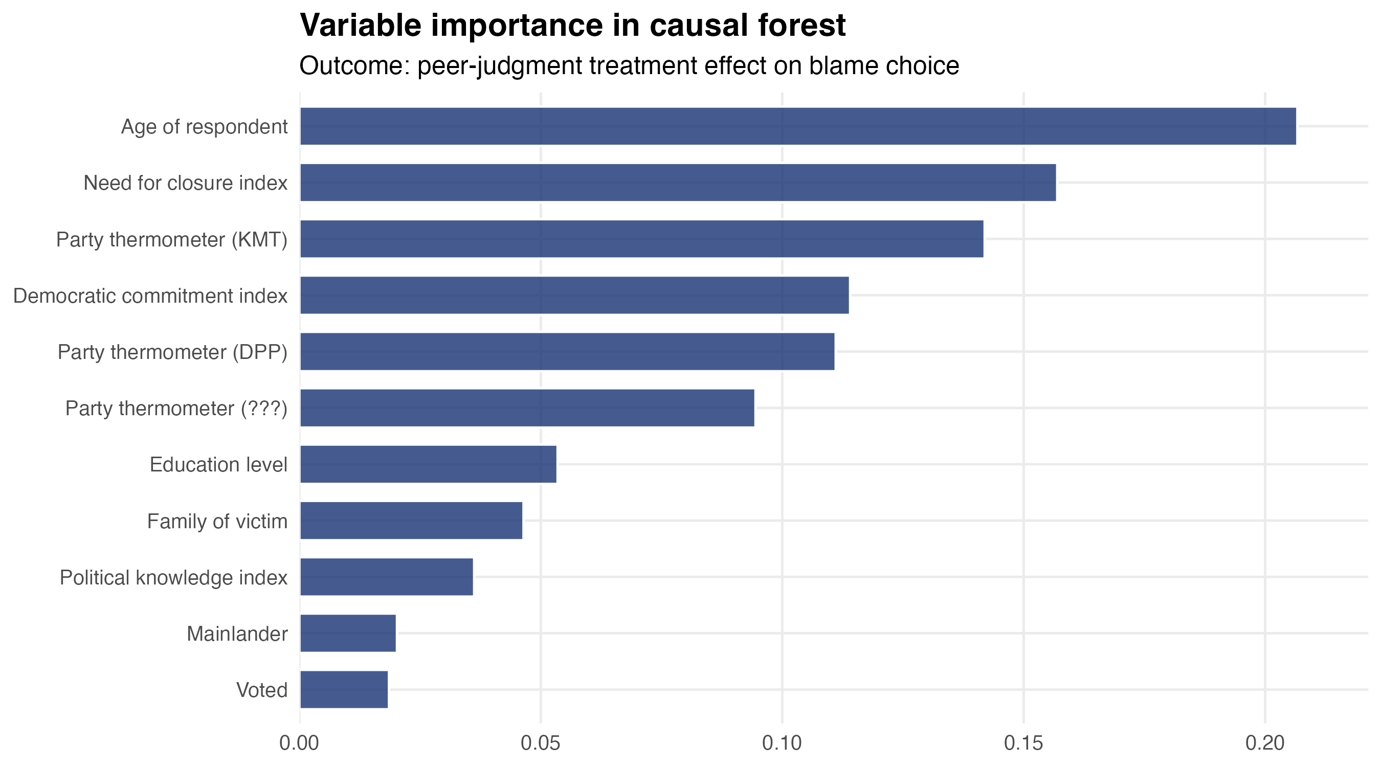
The forest’s verdict: age is the most important moderator, followed by need-for-closure and party-thermometer measures
The age slope: where heterogeneity lives
We can also see how treatment effects vary across our most important variables:
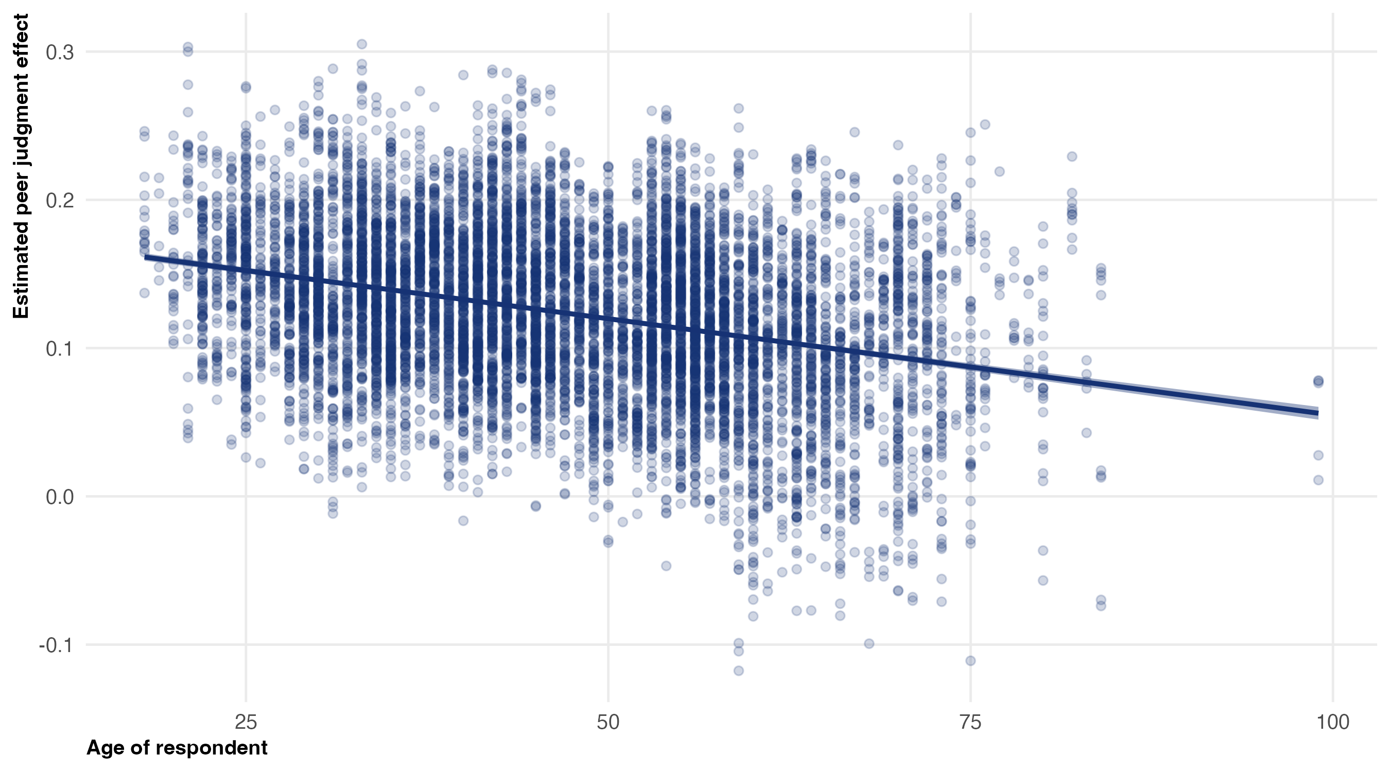
The substantive finding: peer effects are strongest among young respondents (~+0.15 to +0.20 at age 25), declining steadily with age, approaching zero by age 75+. Young people are more susceptible to peer influence on political judgments than older people
What did the forest give us?
Without the forest we’d have run separate subgroup regressions for “young vs old” and “high vs low need-for-closure” and “partisans vs independents” — and each one would have eaten degrees of freedom and inflated the chance of finding spurious patterns
With the forest, we get:
- A ranking of which covariates drive heterogeneity (variable importance)
- A full distribution of \(\hat\tau(X)\) — not one number per subgroup, but an individual estimate per respondent
- A way to plot \(\hat\tau\) against any covariate post-hoc, without pre-specifying interactions
A warning: causal forests aren’t magic. The ATE is causal — treatment was randomized. But the heterogeneity we just discovered is correlational: the moderator variables aren’t randomized
So when the result says “the peer effect is bigger among young respondents,” it doesn’t say why. Maybe younger people are genuinely more susceptible (developmentally). But maybe age correlates with ideology, media consumption, etc.
5. Recap
What we did today
Walked the economist’s path through two causal-inference tools:
| Tool | What it does | Uses what from Week 8? |
|---|---|---|
| Propensity-score matching | Pair treated/control on \(\hat\pi(X)\) | Binary logit (Week 3) |
| Causal forest | Estimate \(\hat\tau(X)\) per observation | Random forest (last week) |
The pattern: every method is built on top of an MLE or ML model we’ve seen. Rather than prediction for its own sake, these approaches are about improving causal inference
There are other applications of MLE/ML to causal inference (e.g., generating strong instruments)
The big assumption (worth repeating)
Everything we did rested on conditional unconfoundedness: once we condition on \(X\), treatment is as good as random. In symbols:
\[Y(0), Y(1) \;\perp\; T \;\big|\; X\]
This is an assumption, not a result. If there’s an unmeasured confounder — anything that drives both treatment and outcome but isn’t in \(X\) — the estimates are biased. PSM and causal forests are both selection-on-observables methods. They cannot help with selection on unobservables
For selection on unobservables you need different tools: instrumental variables, regression discontinuity, difference-in-differences. Those are the topic of POL 214 / a serious causal-inference course