| wall | protestant | age |
|---|---|---|
| 1 | Non-Protestant | 54 |
| 0 | Protestant | 65 |
| 0 | Protestant | 74 |
| 0 | Non-Protestant | 58 |
| 0 | Non-Protestant | 53 |
Maximum Likelihood Estimation
POL 213 · Week 4
Juan F. Tellez
University of California, Davis
April 22, 2026
Housekeeping
- PS3
- Group project check-ins: Ipe ✅
- Midterm next week: blue books
Where we are
Four weeks so far
Week 1: OLS
\[Y = X\beta + \varepsilon\]
Closed-form estimator. Effect of \(X\) = \(\beta\)
Week 2: Transformed OLS
\[Y = f(X)\beta + \varepsilon\]
You chose nonlinearity. Effects depend on where you are
Week 3: Logit
\[\Pr(Y = 1) = \sigma(X\beta)\]
Model imposed nonlinearity. Effect interpretation needs scenarios
Week 4: MLE
glm(Y ~ X, data = data, family = binomial())
Estimating \(\beta\) when there is no closed-form solution
1. Review: the logit workflow
The data (same as Week 3)
2020 Cooperative Election Study — a sample of US adults answering policy questions
- Outcome (
wall): 1 = supports a US–Mexico border wall, 0 = opposes - Predictor of interest (
protestant): 1 = Protestant, 0 = Non-Protestant - Control (
age): in years
Same research question: does being Protestant predict support for a border wall, adjusting for age?
Step 1: glm() returns log-odds coefficients, not effects
Call:
glm(formula = wall ~ protestant + age, family = binomial(link = "logit"),
    data = bot_clean)

Coefficients:
                       Estimate Std. Error z value Pr(>|z|)
(Intercept)          -1.6308850  0.0261699  -62.32   <2e-16 ***
protestantProtestant  0.6973040  0.0181994   38.31   <2e-16 ***
age                   0.0195523  0.0004964   39.39   <2e-16 ***
---
Signif. codes:  0 '***' 0.001 '**' 0.01 '*' 0.05 '.' 0.1 ' ' 1

(Dispersion parameter for binomial family taken to be 1)

    Null deviance: 81318  on 60727  degrees of freedom
Residual deviance: 77682  on 60725  degrees of freedom
AIC: 77688

Number of Fisher Scoring iterations: 4
Those numbers are in log-odds
The linear predictor \(z = X\beta\) is what the model is linear in:
\[\log\!\left(\frac{p}{1-p}\right) \;=\; \beta_0 \;+\; \beta_1 \cdot \text{Protestant} \;+\; \beta_2 \cdot \text{age}\]
So the coefficients are:
- Intercept (\(\hat\beta_0\)): the log-odds of supporting the wall for a non-Protestant aged 0
- Protestant (\(\hat\beta_1\)): how much log-odds shifts when Protestant → 1, holding age fixed
- age (\(\hat\beta_2\)): how much log-odds shifts per year of age, holding religion fixed
Nobody thinks in log-odds. We need to convert to probabilities
Step 2: plug in a scenario, get two probabilities
“Hold age fixed at the sample median; vary Protestant”:
# build a scenario grid
scenario = tibble(
  protestant = factor(c("Non-Protestant", "Protestant"),
                       levels = c("Non-Protestant", "Protestant")),
  age        = median(bot_clean$age, na.rm = TRUE)
)

predictions(mod_wall, newdata = scenario, type = "response") |>
  as_tibble() |>
  select(protestant, age, estimate, conf.low, conf.high)
# A tibble: 2 × 5
protestant age estimate conf.low conf.high
<fct> <dbl> <dbl> <dbl> <dbl>
1 Non-Protestant 49 0.338 0.333 0.343
2 Protestant 49 0.506 0.499 0.513Two numbers with uncertainty. Now in probability units. This is what you report
I switched to predictions()
predictions() and augment() do the same thing, but predictions() give us CI by default
Step 2: visualize the effect
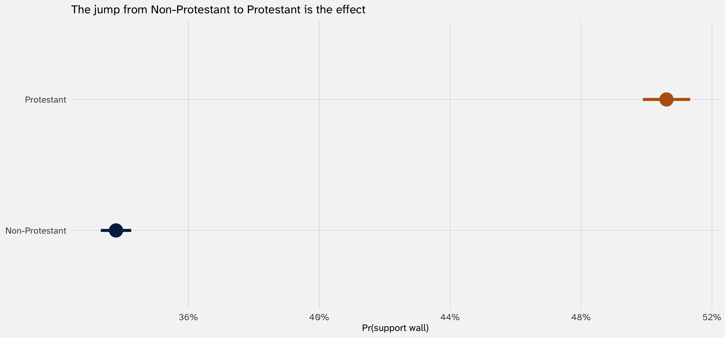
The probabilities come from our log-odds
Our model gives us back log-odds coefficients; how do we get probabilities?
Step 1 is the same as OLS: plug in our \(\beta\) estimates and scenario values into:
\(\log\!\left(\frac{p}{1-p}\right) \;=\; \beta_0 \;+\; \beta_1 \cdot \text{Protestant} \;+\; \beta_2 \cdot \text{age}\)
From the fitted model: \(\hat\beta_0 = -1.63\), \(\hat\beta_1 = 0.7\), \(\hat\beta_2 = 0.02\). Scenario: age = 49 (sample median).
Non-Protestant (Protestant = 0): \[\hat\eta \;=\; -1.63 \;+\; 0.7 \cdot 0 \;+\; 0.02 \cdot 49 \;=\; -0.65\]
Protestant (Protestant = 1): \[\hat\eta \;=\; -1.63 \;+\; 0.7 \cdot 1 \;+\; 0.02 \cdot 49 \;=\; 0.05\]
These are log-odds (\(\eta \;=\; \log\!\frac{p}{1-p}\))
Rounding means these slides won’t look the same
The by-hand example here where we’ve rounded and the R-based slides later won’t match exactly because of rounding
From log-odds to probabilities
Step 2 “Reverse” the log-odds into probabilities:
Solve for \(p\): \[ \eta \;=\; \log\!\frac{p}{1-p} \;\;\Longrightarrow\;\; e^{\eta} \;=\; \frac{p}{1-p} \;\;\Longrightarrow\;\; p \;=\; \frac{e^{\eta}}{1 + e^{\eta}} \;=\; \frac{1}{1 + e^{-\eta}} \]
Plug in log-odds to get back probabilities (\(p\)):
Non-Protestant (\(\hat\eta = -0.65\)): \[\hat p \;=\; \frac{1}{1 + e^{-\hat\eta}} \;=\; \frac{1}{1 + e^{-(-0.65)}} \;=\; \frac{1}{1 + e^{0.65}} \;\approx\; 0.34\]
Protestant (\(\hat\eta = 0.05\)): \[\hat p \;=\; \frac{1}{1 + e^{-\hat\eta}} \;=\; \frac{1}{1 + e^{-(0.05)}} \;\approx\; 0.51\]
In R
The fitted values of \(\widehat{\eta}\) are sometimes referred to as being on the “link” scale:
 Estimate Std. Error      z Pr(>|z|)   S    2.5 %  97.5 %
  -0.6728     0.0106 -63.62   <0.001 Inf -0.69355 -0.6521
   0.0245     0.0148   1.66   0.0973 3.4 -0.00446  0.0534

Type: link
The fitted values of \(\widehat{p}\) are sometimes referred to as being on the “response” scale:
 Estimate Std. Error   z Pr(>|z|)   S 2.5 % 97.5 %
    0.338    0.00237 143   <0.001 Inf 0.333  0.343
    0.506    0.00369 137   <0.001 Inf 0.499  0.513

Type: response
Remember \(\eta \rightarrow p\)
You can move from one to the other by passing through the sigmoid
Step 3: the marginal effect is different at every age
The marginal effect of being Protestant is not one number. It depends on other covariates (age), because they shift where you are on the sigmoid
 age Estimate Std. Error    z Pr(>|z|)      S 2.5 % 97.5 %
  25    0.149    0.00415 35.8   <0.001  929.7 0.141  0.157
  45    0.166    0.00437 38.0   <0.001 1048.2 0.157  0.175
  65    0.173    0.00442 39.1   <0.001    Inf 0.164  0.181

Term: protestant
Type: response
Comparison: Protestant - Non-Protestant
Same \(\hat\beta\). Three different ME values. The nonlinearity scales everything.
The AME — one number for the paper
Average the ME across the observed sample:
 Estimate Std. Error  z Pr(>|z|)      S 2.5 % 97.5 %
    0.164    0.00431 38   <0.001 1046.6 0.155  0.172

Term: protestant
Type: response
Comparison: Protestant - Non-Protestant
One probability-scale number. This is the headline quantity → Comparing respondents of the same age, Protestants are 16.4 percentage points more likely to support building “the wall” than non-Protestants
Which scenarios does the AME cover?
The AME averages over the scenarios your data actually exhibits — not a made-up profile. Since the ME estimates what happens when you shift \(X\) while holding \(Z\) constant, you can have as many as one distinct ME per unique combination of \(Z\) in your data
The logit workflow: fit, convert, report
- Fit:
glm(Y ~ X + controls, family = binomial) - Don’t report raw coefficients as the effect (they’re log-odds); leave table in appendix
- Plot predicted probabilities across your key predictor, holding controls at sensible values
- Report the AME as your top-level number; show scenarios for interpretation
- Always state which scenario or average you used
An interesting question from last time: why does the effect of \(X\) depend on \(Z\), even though we didn’t put an interaction in the model?
2. The puzzle: no interaction, yet Z still moderates
Restating the puzzle
From the previous slide, model returns three different ME values:
 age Estimate Std. Error    z Pr(>|z|)      S 2.5 % 97.5 %
  25    0.149    0.00415 35.8   <0.001  929.7 0.141  0.157
  45    0.166    0.00437 38.0   <0.001 1048.2 0.157  0.175
  65    0.173    0.00442 39.1   <0.001    Inf 0.164  0.181

Term: protestant
Type: response
Comparison: Protestant - Non-Protestant
But the model we fit was additive:
\[\log\!\left(\frac{p}{1-p}\right) \;=\; \beta_0 + \beta_1 \cdot \text{Protestant} + \beta_2 \cdot \text{age}\]
There is no \(\text{Protestant} \times \text{age}\) term. So where did the age-dependence come from?
Two scales, two answers
The model lives on two scales — log-odds (what the linear predictor produces) and probability (what we care about)
Log-odds scale
What the coefficients are in
\[\eta \;=\; \beta_0 + \beta_1 X + \beta_2 Z\]
Linear. Additive in \(X\) and \(Z\)
Probability scale
What you report
\[p \;=\; \sigma(\eta)\]
Nonlinear. S-shaped in \(\eta\)
The question “does the effect of \(X\) depend on \(Z\)?” has a different answer on each scale
On the log-odds scale, the effect of \(X\) is constant
Take the derivative of \(\eta\) with respect to \(X\):
\[\eta \;=\; \beta_0 + \beta_1 X + \beta_2 Z \;\;\Longrightarrow\;\; \frac{\partial \eta}{\partial X} \;=\; \beta_1\]
\(\beta_1\) does not depend on \(Z\). On the log-odds scale, the additive model is just OLS: one slope, same for everyone
So if you interpret coefficients in log-odds units, there’s no puzzle. \(\beta_1\) is \(\beta_1\)
On the probability scale, the effect of \(X\) scales with \(p(1-p)\)
Chain rule from Week 3:
\[\frac{\partial p}{\partial X} \;=\; \underbrace{\frac{\partial p}{\partial \eta}}_{\sigma'(\eta) \,=\, p(1-p)} \;\cdot\; \underbrace{\frac{\partial \eta}{\partial X}}_{\beta_1} \;=\; p(1-p) \cdot \beta_1\]
The slope of the sigmoid \(p(1-p)\) depends on \(\eta\), and \(\eta\) depends on \(Z\)
So: \(Z\) shifts \(\eta\) → \(\eta\) shifts \(p\) → \(p\) shifts \(p(1-p)\) → \(p(1-p)\) scales the ME of \(X\)
The “dependence on \(Z\)” enters only through the sigmoid’s curvature
By hand: three ages, three MEs
For our fitted model, at a non-Protestant baseline:
\[\hat\eta \;=\; \hat\beta_0 \;+\; \hat\beta_1 \cdot \text{Protestant} \;+\; \hat\beta_2 \cdot \text{age} \qquad\qquad \hat p \;=\; \frac{1}{1 + e^{-\hat\eta}}\]
coefs = coef(mod_wall)

tibble(age = c(25, 45, 65), protestant = 0, beta_1 = coefs["protestantProtestant"]) |>
  mutate(
    eta     = coefs["(Intercept)"] + coefs["protestantProtestant"] * protestant + coefs["age"] * age,
    p       = 1 / (1 + exp(-eta)),
    scaling = p * (1 - p),
    ME      = coefs["protestantProtestant"] * scaling
  )
# A tibble: 3 × 7
age protestant beta_1 eta p scaling ME
<dbl> <dbl> <dbl> <dbl> <dbl> <dbl> <dbl>
1 25 0 0.697 -1.14 0.242 0.183 0.128
2 45 0 0.697 -0.751 0.321 0.218 0.152
3 65 0 0.697 -0.360 0.411 0.242 0.169Same \(\hat\beta_1\). Three different MEs. The only thing that changed is \(p(1-p)\), driven by age sliding you along the sigmoid
The sigmoid’s moderation is highly constrained
So the effect of \(X\) on \(Y\) can depend on \(Z\) through \(p(1-p)\), but in a limited way
Some things the \(p(1-p)\) scaling cannot do:
1. Flip sign — \(p(1-p) > 0\) always, so the ME of \(X\) has the same sign as \(\beta_1\) everywhere
2. Be asymmetric — \(p(1-p)\) is symmetric around \(p = 0.5\). The ME at \(p = 0.2\) equals the ME at \(p = 0.8\)
So the sigmoid does produce moderation → but of a specific, predictable shape. If your theory predicts moderation of a different shape, the sigmoid can’t deliver it
Enter the product term: let \(Z\) move the log-odds slope
Add \(X \cdot Z\) to the linear predictor:
\[\eta \;=\; \beta_0 + \beta_1 X + \beta_2 Z + \beta_3 (X \cdot Z)\]
Take the derivative again:
\[\frac{\partial \eta}{\partial X} \;=\; \beta_1 + \beta_3 Z\]
Now \(Z\) moderates \(X\) on the log-odds scale itself — before the sigmoid ever gets applied
Which means on the probability scale:
\[\frac{\partial p}{\partial X} \;=\; p(1-p) \cdot (\beta_1 + \beta_3 Z)\]
Two sources of \(Z\)-dependence, stacked: one from curvature (\(p(1-p)\)), one from structure (\(\beta_3 Z\))
Fit the interaction, read the product-term coefficient
# A tibble: 4 × 5
  term                     estimate std.error statistic   p.value
  <chr>                       <dbl>     <dbl>     <dbl>     <dbl>
1 (Intercept)              -1.60     0.0312      -51.3  0
2 protestantProtestant      0.596    0.0568       10.5  8.78e- 26
3 age                       0.0189   0.000609     31.0  3.18e-211
4 protestantProtestant:age  0.00197  0.00105       1.88 6.06e-  2
The protestantProtestant:age row is \(\hat\beta_3\) — how the log-odds effect of being Protestant changes per year of age. A real, structural moderation, separate from the sigmoid curvature
The diagnostic: plot ME of \(X\) vs \(Z\) for both models
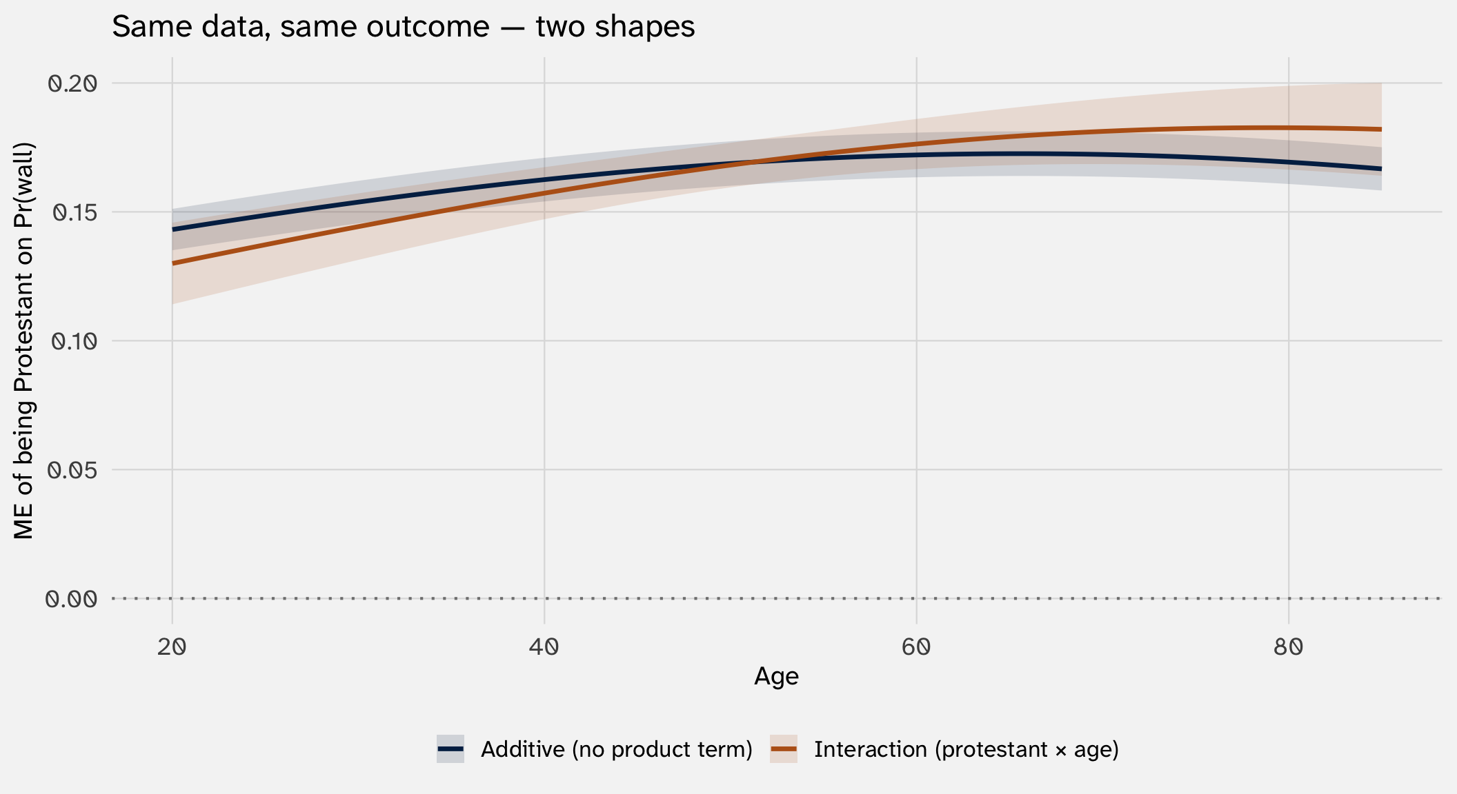
The additive curve can only bend one way. The interaction curve can slope, flip, or cross zero. If the second plot shape matters for your theory, the additive model can’t represent it
In this case, the interaction doesn’t change the curve much; why?
When to include a product term
Include it if your theory says the effect of X depends on Z
3. The framework: maximum likelihood
Open the hood on glm()
Where did \(\hat\beta\) come from?
When we fit a logit model we get back:
Call:
glm(formula = wall ~ protestant + age, family = binomial(link = "logit"),
    data = bot_clean)

Coefficients:
                       Estimate Std. Error z value Pr(>|z|)
(Intercept)          -1.6308850  0.0261699  -62.32   <2e-16 ***
protestantProtestant  0.6973040  0.0181994   38.31   <2e-16 ***
age                   0.0195523  0.0004964   39.39   <2e-16 ***
---
Signif. codes:  0 '***' 0.001 '**' 0.01 '*' 0.05 '.' 0.1 ' ' 1

(Dispersion parameter for binomial family taken to be 1)

    Null deviance: 81318  on 60727  degrees of freedom
Residual deviance: 77682  on 60725  degrees of freedom
AIC: 77688

Number of Fisher Scoring iterations: 4- An estimate \(\hat\beta\)
- A standard error
- A \(z\)-statistic and \(p\)-value
- A “deviance”
- A note:
Number of Fisher Scoring iterations: 4
How are these quantities being estimated/calculated?
OLS is the lucky case: a closed-form solution
In OLS we minimize SSR, take derivatives with respect to \(\beta_0\) and \(\beta_1\), and set them to zero:
\[\frac{\partial \text{SSR}}{\partial \beta_0} \;=\; -2\sum_{i=1}^n (Y_i - \beta_0 - \beta_1 X_i) \;=\; 0\]
\[\frac{\partial \text{SSR}}{\partial \beta_1} \;=\; -2\sum_{i=1}^n X_i(Y_i - \beta_0 - \beta_1 X_i) \;=\; 0\]
Two equations, two unknowns. Solve algebraically:
\[\hat\beta_1 \;=\; \frac{\sum_i (X_i - \bar X)(Y_i - \bar Y)}{\sum_i (X_i - \bar X)^2} \qquad \hat\beta_0 \;=\; \bar Y - \hat\beta_1 \bar X\]
Plug in your data, get the answer. This is rare. Most estimators in statistics don’t have closed forms. OLS is a mathematical “coincidence” — assumptions + SSR line up just right
Same thing in matrix form
With \(k\) predictors, those two equations become \(k+1\) equations — tedious to write out. Matrix notation compresses them to one line: \(\hat\beta = (X'X)^{-1}X'Y\). Same math, compact form. That’s the version you’ll see in textbooks.
Logit has no closed form
Try the same trick. Logit has its own version of OLS’s normal equations — take derivatives, set them to zero:
\[\sum_{i=1}^n \left(Y_i - \frac{1}{1 + e^{-(\beta_0 + \beta_1 X_i)}}\right) \;=\; 0\]
\[\sum_{i=1}^n X_i\!\left(Y_i - \frac{1}{1 + e^{-(\beta_0 + \beta_1 X_i)}}\right) \;=\; 0\]
Two equations, two unknowns — same structure as OLS. But now the sigmoid sits between \(\beta\) and the residual. You can’t isolate \(\beta_0, \beta_1\) algebraically
So we need a different strategy: maximize the likelihood numerically
Maximum Likelihood Estimation: find the \(\beta\) that makes your data most likely
The OLS principle: among all possible \(\beta\) values, pick the one that minimizes the squared distances from \(Y\)
The MLE principle: among all possible \(\beta\) values, pick the one that assigns the highest probability to the \(Y\) values you actually observed
Concretely: we want \(p\) close to \(Y\) for every row.
| protestant | age | wall | p |
|---|---|---|---|
| Non-Protestant | 54 | 1 | ??? |
| Protestant | 65 | 0 | ??? |
| Protestant | 74 | 0 | ??? |
| Non-Protestant | 58 | 0 | ??? |
| Non-Protestant | 53 | 0 | ??? |
When wall = 1, we want the model to assign a big value of \(p\). When wall = 0, we want a small value of \(p\).
MLE’s job: find the \(\beta\) that does this “best” across all rows simultaneously
Specify the likelihood of an observation
For a logit model, the probability of a single observation:
\[\Pr(Y_i \mid X_i, \beta) \;=\; p_i^{Y_i} (1 - p_i)^{1 - Y_i}, \qquad p_i = \sigma(X_i'\beta)\]
This is just the Bernoulli: \(Y_i\) is binary, so its distribution is Bernoulli with parameter \(p_i\) — and \(p_i\) depends on the \(\beta\) we’re estimating.
Reads as: “probability \(p_i\) if \(Y_i = 1\), probability \(1 - p_i\) if \(Y_i = 0\)” — the Bernoulli formula from Week 3
The logit likelihood is a product of Bernoulli terms
What is the probability of observing all of our data?
Observations are independent, so the probability of the whole dataset is the product:
\[\mathcal{L}(\beta) \;=\; \prod_{i=1}^n p_i^{Y_i} (1 - p_i)^{1 - Y_i}\]
\(\mathcal{L}(\beta)\) is a function of \(\beta\) — as \(\beta\) changes, the \(p_i\)’s change, and so does the product
MLE principle: find the \(\hat\beta\) that maximizes \(\mathcal{L}\). That’s the value of \(\beta\) that best “explains” the data we saw
Independence is an assumption
The product form only works if observations are independent (given \(X\) and \(\beta\)). With clustered data — panel, students in schools, voters in precincts — the joint probability doesn’t factor this way. Point estimates are often still consistent, but standard errors are too small
Take logs: products become sums
Products are hard to differentiate; sums are easy. Take the log:
\[\ell(\beta) \;=\; \log \mathcal{L}(\beta) \;=\; \sum_{i=1}^n \Bigl[ Y_i \log p_i + (1 - Y_i) \log(1 - p_i) \Bigr]\]
\(\log\) is monotonic — the \(\beta\) that maximizes \(\mathcal{L}\) also maximizes \(\ell\). But \(\ell\) is a sum, which makes the derivatives tractable
From now on we always work with the log-likelihood \(\ell(\beta)\)
Maximize by climbing: Newton–Raphson walks to the peak
We can’t solve for \(\hat\beta\) directly. So we search for it:
- Start at a guess \(\beta^{(0)}\)
- Compute the slope (gradient) and curvature (Hessian) of \(\ell\) at the guess
- Use them to jump to a better \(\beta^{(1)}\)
- Repeat until the jumps stop
This is Newton–Raphson (also: Fisher scoring). Each iteration climbs the log-likelihood surface
Let’s see how to recover the estimates from this simple model:
Call:
glm(formula = wall ~ protestant, family = binomial, data = bot_clean)

Coefficients:
                     Estimate Std. Error z value Pr(>|z|)
(Intercept)          -0.70622    0.01043  -67.69   <2e-16 ***
protestantProtestant  0.80345    0.01782   45.08   <2e-16 ***
---
Signif. codes:  0 '***' 0.001 '**' 0.01 '*' 0.05 '.' 0.1 ' ' 1

(Dispersion parameter for binomial family taken to be 1)

    Null deviance: 81318  on 60727  degrees of freedom
Residual deviance: 79270  on 60726  degrees of freedom
AIC: 79274

Number of Fisher Scoring iterations: 4
Searching for \(\beta_1\)
The log-likelihood is just a function we evaluate. Plug in a \(\beta_1\), get a number — how probable the observed data is under that \(\beta_1\).
Remember \[p = \frac{1}{1 + e^{-(\beta_0 + \beta_1 Protestant)}}\]
and
\[\ell(\beta) = \sum_{i=1}^n \Bigl[ Y_i \log p_i + (1 - Y_i) \log(1 - p_i) \Bigr]\]
Plug in a \(\beta_1\), compute \(\ell\)
Let’s search just for \(\beta_1\), pretending we already know \(\hat\beta_0\)
# A tibble: 6 × 2
     b1 log_lik
  <dbl>   <dbl>
1  -1   -46730.
2  -0.5 -43520.
3   0   -41161.
4   0.3 -40241.
5   0.7 -39661.
6   1.5 -40762.
As with the sum of squared residuals, we don’t care about the raw numbers:
- it’s unit-less. It’s the sum of the log of the probabilities of observing each row
- Absolute value is nearly meaningless. \(-46{,}730\) is big-looking because it’s a sum over thousands of observations
- All we care is that some \(\beta_1\) values make the data more probable than others. Which one makes it most probable? That’s MLE
The log-likelihood is a curve we want to climb
Evaluate \(\ell\) on a fine grid of \(\beta_1\) values and plot:
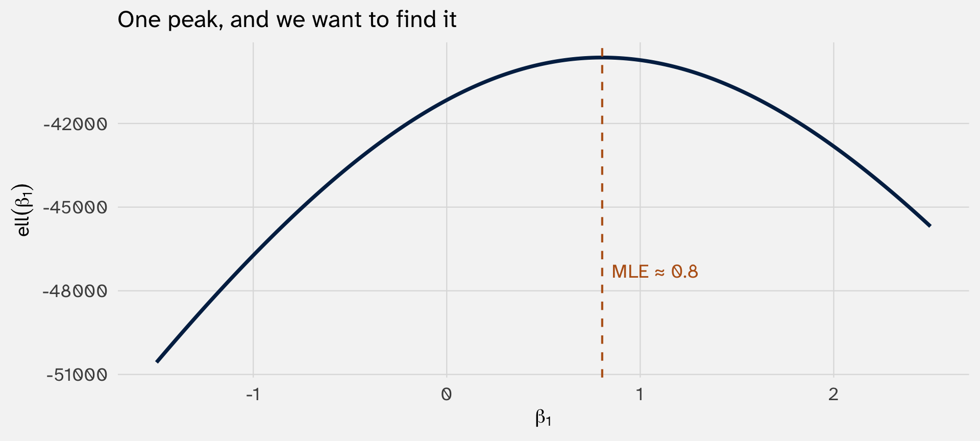
The peak’s location is what glm() prints as \(\hat\beta_1\). But we don’t have its coordinates yet — we have to search.
Start at a guess, see how high you are
Pick any starting value — say \(\beta_1^{(0)} = -0.5\). Evaluate \(\ell\) there.
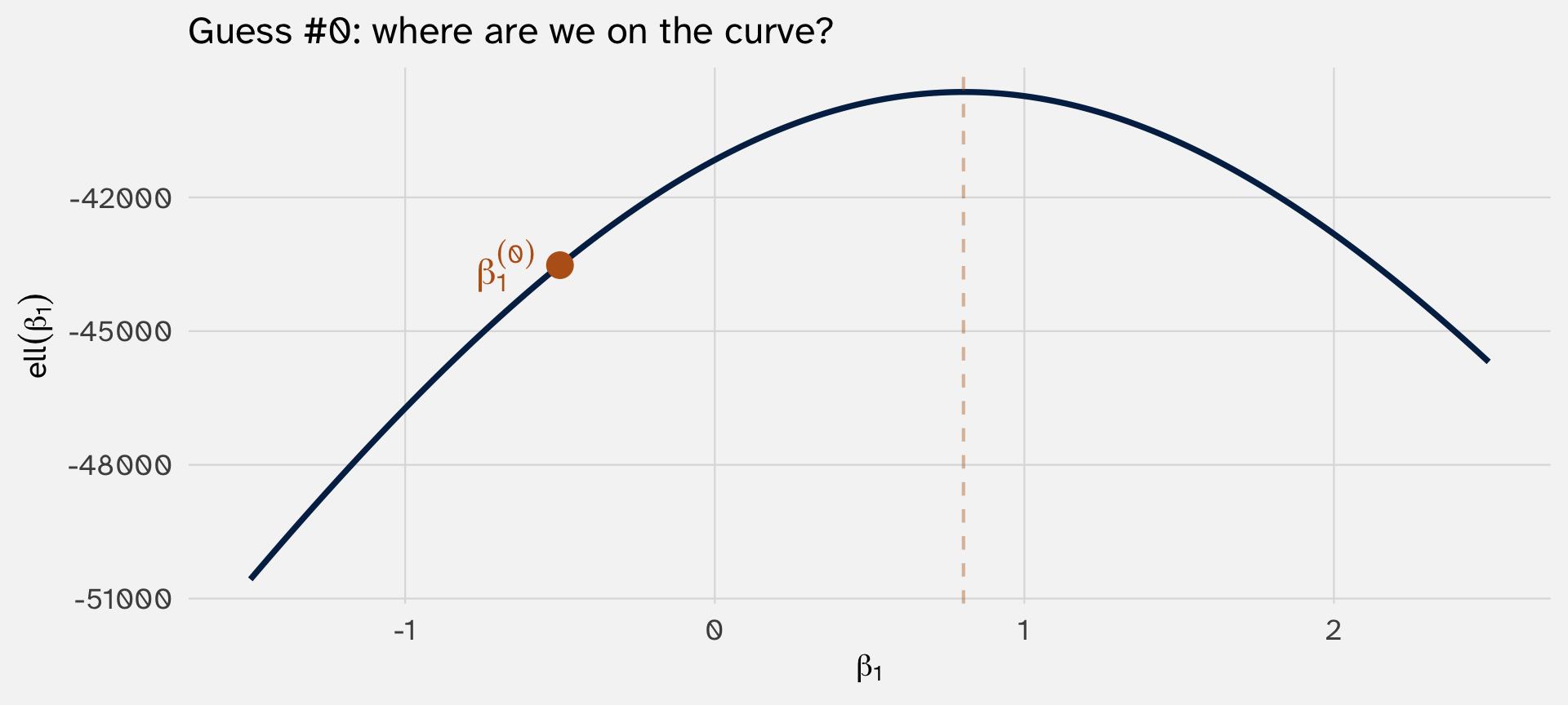
We’re at \((\beta_1^{(0)}, \ell(\beta_1^{(0)}))\). Remember we can’t see the MLE; is it to the right, or left of us? How far is it?
Gradient: one nudge tells us direction
At \(\beta_1^{(0)} = -0.5\), which way should we step? Evaluate \(\ell\) twice — once at our current \(\beta_1\), once a tiny step to the right:
# A tibble: 2 × 3
     b1      ll slope
  <dbl>   <dbl> <dbl>
1 -0.5  -43520.   NA
2 -0.49 -43464. 5628.
Positive slope → step right. (Negative → step left.)
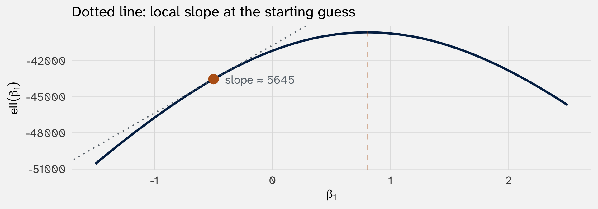
Hessian: how fast the slope itself is changing
How big a step? That depends on how fast the slope is itself changing
Apply the same nudge trick one level up — three evaluations of \(\ell\) give us two slopes, which give us one Hessian:
# A tibble: 3 × 4
     b1      ll slope hessian
  <dbl>   <dbl> <dbl>   <dbl>
1 -0.5  -43520.   NA      NA
2 -0.49 -43464. 5628.     NA
3 -0.48 -43408. 5594.  -3424.
Big |Hessian| → slope drops to zero quickly as \(\beta\) moves → peak is nearby → take a small step
Small |Hessian| → slope changes slowly as \(\beta\) moves → peak is far away → take a big step
Take the step: Newton–Raphson in action
Newton–Raphson combines gradient and Hessian into one update:
\[\beta_1^{(1)} \;=\; \beta_1^{(0)} \;-\; \frac{\ell'(\beta_1^{(0)})}{\ell''(\beta_1^{(0)})}\]
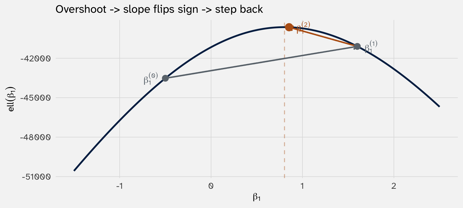
We overshot. But at \(\beta_1^{(1)}\) the slope is now negative — so the next step is leftward. Each iteration recomputes slope + curvature at the new point, so mistakes self-correct.
Arriving at the MLE estimates
After a handful of iterations, slope → 0, step size → 0, and \(\beta_1^{(k)}\) converges on the MLE. That’s what Fisher Scoring iterations: 4 means: the algorithm did this loop four times before the steps got negligibly small
glm() doesn’t actually nudge
In practice we don’t compute the Hessian by finite differences. For logit there’s a formula:
\[\ell''(\beta_1) \;=\; -\sum_i X_i^2 \, p_i(1-p_i)\]
Plug in the current \(\beta_1\), get a number. That’s what glm() does internally. The finite-difference picture is the intuition; the formula is the computation.
The log-likelihood surface has one peak (usually)
Same idea when estimating \(\beta_0\) and \(\beta_1\) simultaneously, but in 3D space
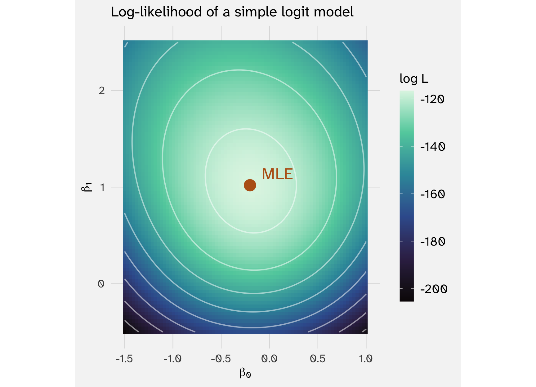
One hill, one summit. MLE is the point on the ridge
In simulation, MLE recovers the true \(\beta\)
# A tibble: 1 × 5
  term  estimate std.error statistic  p.value
  <chr>    <dbl>     <dbl>     <dbl>    <dbl>
1 X         1.12     0.123      9.14 6.16e-20
True \(\beta = 1.2\). MLE estimate: about \(1.12 \pm 0.12\). The recipe works. This is the claim underneath everything glm() does
plogis() for the sigmoid
Instead of writing (1 + exp(-beta_true * X) we could use plogis(beta_true * X)
The log-likelihood is concave: one peak, no ridges, no valleys
For logit (and for most MLE problems), the log-likelihood is concave — curved downward everywhere
Why it matters:
- One maximum: no risk of Newton–Raphson finding a local peak and missing the global one
- Convergence: from any starting point, the climber will reach the summit
- Unique \(\hat\beta\): if estimation succeeds, the answer is the answer
This is why glm() usually converges in 4–5 iterations. The surface is well-behaved
OLS is MLE under Gaussian errors
A nice, encouraging property of MLE is that we can use it to recover OLS estimates:
If you assume \(Y_i = X_i'\beta + \varepsilon_i\) with \(\varepsilon_i \sim N(0, \sigma^2)\), the likelihood is:
\[\mathcal{L}(\beta, \sigma^2) \;=\; \prod_i \frac{1}{\sqrt{2\pi\sigma^2}} \exp\!\left(-\frac{(Y_i - X_i'\beta)^2}{2\sigma^2}\right)\]
Take the log, drop constants. Maximizing \(\ell\) reduces to:
\[\min_\beta \;\sum_i (Y_i - X_i'\beta)^2\]
That’s least squares. OLS is not really a different estimator → it’s MLE under the Gaussian assumption
glm(Y ~ X, family = gaussian) and lm(Y ~ X) return identical coefficients. Try it
Standard errors also depend on the likelihood
Once we’ve found \(\hat\beta\), how precisely do we know it? That depends on the curvature of \(\ell\) at the peak
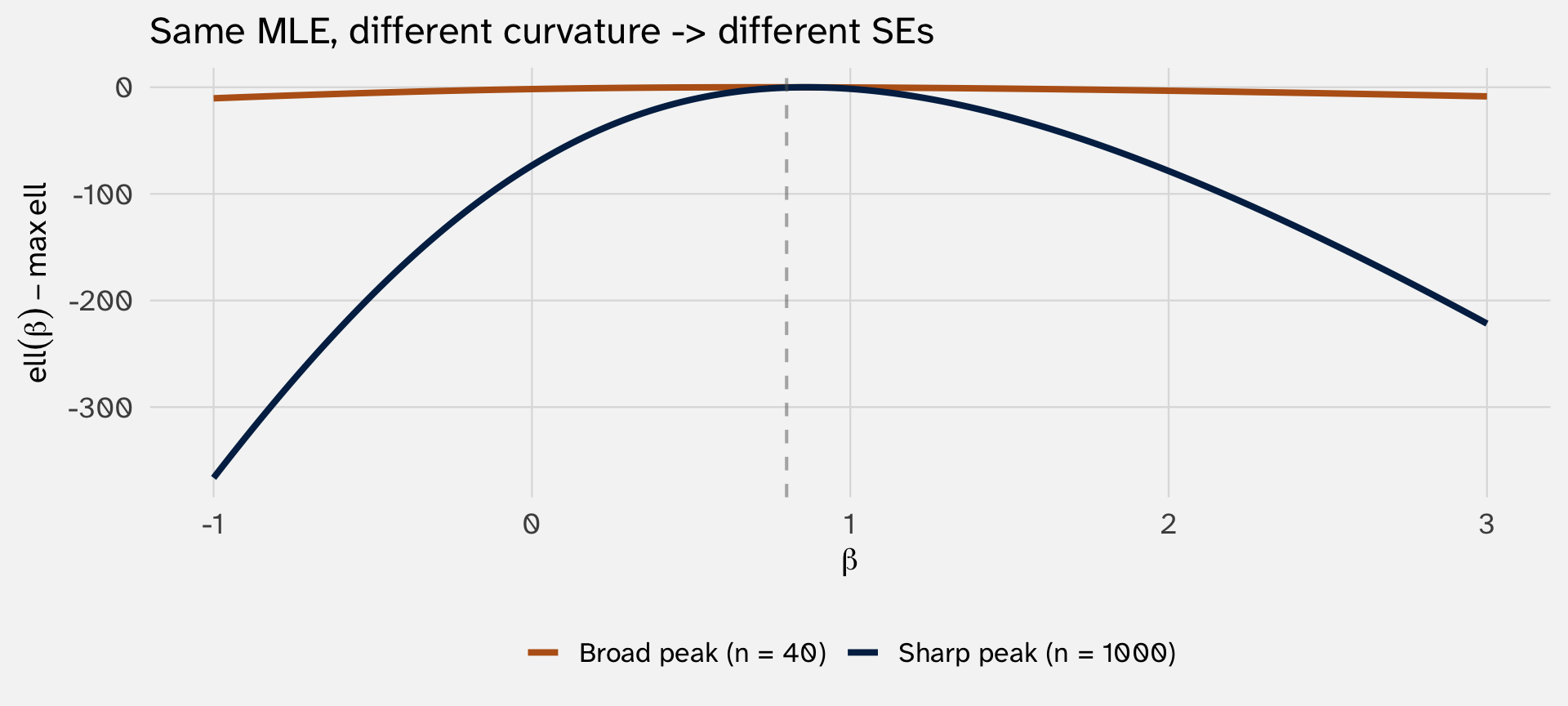
Sharp peak → small changes in \(\beta\) fit much worse → \(\hat\beta\) is precise.
Broad peak → many \(\beta\) values fit nearly as well → \(\hat\beta\) is uncertain.
We call this curvature the Fisher information: \(\mathcal{I}(\hat\beta) \;=\; -\,\ell''(\hat\beta)\) → the negative second derivative of \(\ell\)
From Fisher information to standard errors
Information and variance are inverses. More information about \(\beta\) → less uncertainty → smaller variance. Big \(\mathcal{I}\) gives narrow error bars, not wide ones
For one parameter:
\[\text{Var}(\hat\beta) \;\approx\; \frac{1}{\mathcal{I}(\hat\beta)} \qquad \text{SE}(\hat\beta) \;\approx\; \frac{1}{\sqrt{\mathcal{I}(\hat\beta)}}\]
For multiple parameters (matrix case): invert the matrix, take the square root of the diagonal:
\[\text{SE}(\hat\beta_j) \;=\; \sqrt{\bigl[\mathcal{I}(\hat\beta)^{-1}\bigr]_{jj}}\]
MLE theorem (large-sample): \(\hat\beta \stackrel{a}{\sim} N\!\left(\beta, \,\mathcal{I}(\beta)^{-1}\right)\) — approximately normal, centered at the truth, with covariance set by the peak’s curvature. This is where \(z\)-statistics and confidence intervals come from.
By hand: SE from three evaluations at \(\hat\beta\)
Same three-evaluations trick as before — just applied at the peak instead of at a starting guess.
- Before (Newton–Raphson): evaluate at \(\beta_1^{(0)}\) to decide where to step
- Now (Fisher info): evaluate at \(\hat\beta_1\) to measure how sharp the peak is
b1_mle  = coef(glm(Y ~ X, family = binomial))[2]
epsilon = 0.01

tibble(
  b1 = c(b1_mle, b1_mle + epsilon, b1_mle + 2 * epsilon),
  ll = c(log_lik(b1_mle),
         log_lik(b1_mle + epsilon),
         log_lik(b1_mle + 2 * epsilon))
) |>
  mutate(slope   = (ll - lag(ll))       / epsilon,
         hessian = (slope - lag(slope)) / epsilon,
         fisher  = -hessian,            # Fisher info = -Hessian
         se      = 1 / sqrt(fisher))    # SE = 1/√I
# A tibble: 3 × 6
b1 ll slope hessian fisher se
<dbl> <dbl> <dbl> <dbl> <dbl> <dbl>
1 1.12 -314. NA NA NA NA
2 1.13 -314. 7.55 NA NA NA
3 1.14 -314. 6.90 -64.8 64.8 0.124From Fisher info to standard error
b1_mle  = coef(glm(Y ~ X, family = binomial))[2]
epsilon = 0.01

tibble(
  b1 = c(b1_mle, b1_mle + epsilon, b1_mle + 2 * epsilon),
  ll = c(log_lik(b1_mle),
         log_lik(b1_mle + epsilon),
         log_lik(b1_mle + 2 * epsilon))
) |>
  mutate(slope   = (ll - lag(ll))       / epsilon,
         hessian = (slope - lag(slope)) / epsilon,
         fisher  = -hessian,            # Fisher info = -Hessian
         se      = 1 / sqrt(fisher))    # SE = 1/√I
# A tibble: 3 × 6
b1 ll slope hessian fisher se
<dbl> <dbl> <dbl> <dbl> <dbl> <dbl>
1 1.12 -314. NA NA NA NA
2 1.13 -314. 7.55 NA NA NA
3 1.14 -314. 6.90 -64.8 64.8 0.124Compare to glm():
Our by-hand SE is close, not exact
glm() works with the full Fisher information matrix (one row/column per parameter), inverts it, and reads each SE off the diagonal. Our scalar recipe only varies \(\beta_1\) — treating \(\hat\beta_0\) as known. The difference: glm() accounts for uncertainty in \(\hat\beta_0\) leaking into uncertainty about \(\hat\beta_1\), since the two are correlated in how they fit the data. Our by-hand SE ignores that coupling — technically it’s a profile SE.
4. When logit breaks: convergence and separation
Failure modes that reveal how MLE works under the hood
How glm() knows it’s done
Newton–Raphson keeps iterating until the log-likelihood stops meaningfully improving.
glm()’s stopping rule (the default):
- After each iteration, check whether the deviance (\(-2\ell\)) changed by less than \(10^{-8}\) (relative)
- If yes → converged. Print
Fisher Scoring iterations: kand stop - If 25 iterations pass without this check firing → give up. Print
algorithm did not converge
Three things could make this check fire (all equivalent at the MLE):
- Gradient near zero: slope is flat → we’re on the peak
- Step size near zero: the update \(\beta - \ell'/\ell''\) barely moves us
- Log-likelihood change near zero: we’re not improving anymore
glm() uses the third.
When the warning fires, it’s diagnostic — not random. Something about your data is preventing Newton–Raphson from reaching a peak. Three distinct geometries can cause this →
Three geometries, three reasons
The log-likelihood surface has no clean peak when:
1. No peak — peak at infinity → perfect separation. \(\hat\beta \to \infty\); we’ll work through this next.
2. Ridge, not summit — peak not unique → severe collinearity. Two predictors move together; only their sum is identifiable.
3. Flat surface — not enough curvature → weak identification. Tiny sample, too many parameters, or outcome nearly constant.
All three say the same thing: something about your data + your specification don’t pin down \(\beta\). None of these mean your theory or causal identification strategy is wrong: a bad theory/causal ID can converge without problem
A small-N dataset with a suspiciously clean predictor
Suppose you’re studying which post-communist countries transitioned to democracy by 2000. You have \(n = 40\) countries and one predictor: did the country join the EU?
     0  1
  0 25  0
  1  0 15
Every EU-joiner democratized. Every non-joiner didn’t. Joining the EU perfectly explains which countries democratized
Fitting logit returns absurd coefficients and SEs
Call:
glm(formula = democratic ~ joined_eu, family = binomial(link = "logit"),
    data = transitions)

Coefficients:
             Estimate Std. Error z value Pr(>|z|)
(Intercept)    -26.57   71224.80       0        1
joined_eu       53.13  116309.62       0        1

(Dispersion parameter for binomial family taken to be 1)

    Null deviance: 5.2925e+01  on 39  degrees of freedom
Residual deviance: 2.3206e-10  on 38  degrees of freedom
AIC: 4

Number of Fisher Scoring iterations: 25
\(\hat\beta_1 \approx 53.1\), SE ≈ 116,310. The coefficient is huge, the uncertainty is absurd.
And glm() didn’t even warn us. With larger samples it would warn. The nonsensical SEs are your signal, not the warning.
This is perfect separation. The predictor partitions the outcome with zero error
Why: the log-likelihood has no finite maximum
For every value of \(\beta\), a larger \(\beta\) fits the data better. The log-likelihood keeps climbing
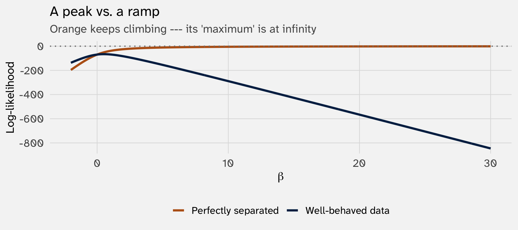
Blue: a unique \(\hat\beta\) maximizes the log-likelihood. Orange: the “maximum” is at \(+\infty\). There is no \(\hat\beta\)
Separation can happen with more than one \(X\)
Separation exists if some linear combination of predictors perfectly splits \(Y\). “Single-predictor” separation (our EU example) is one instance; “joint” separation — caused by a combination of \(X\) — is sneakier and harder to diagnose by eyeballing the data.
Separation should make you question your theory
Methods textbooks say: drop the variable, penalize, collect more data. Fine for a data-driven approach (e.g., some machine-learning applications). But if your model encodes a causal argument, “just drop \(X\)” isn’t on the table → separation is telling you something more interesting than “this dataset misbehaves.”
1. Question your theory. If every Republican voted yes, what is “Republican vs. Democrat” actually explaining? The predictor perfectly matches \(Y\) — so it’s a restatement, not an explanation. A variable that discriminates perfectly has nothing left to model.
2. Question your data. Is your sample censored or selected? Crossover cases might exist in the population but got filtered out — missing values, “unclassified” rows, refusals. Check what you dropped.
3. Question whether quant methods fit. If the pattern really is in the phenomenon — not just in a bad sample — then the question may not be a regression question. Case studies, process tracing, or a qualitative comparison may fit better. Forcing a logit on invariant data won’t manufacture insight.
Four answers
Opening slide asked:
1. Why not \((X'X)^{-1}X'Y\) anymore?
→ Logit’s likelihood equations are nonlinear. No closed form exists
2. Why does glm() print “iterations: 4”?
→ Newton–Raphson climbing the log-likelihood surface
3. Why do the SEs look like \(\sqrt{\text{diag}(\mathcal{I}^{-1})}\)?
→ Asymptotic normality: \(\hat\beta \sim N(\beta, \mathcal{I}^{-1})\)
4. Why does the model sometimes fail with “fitted probabilities numerically 0 or 1”?
→ Perfect separation: the log-likelihood has no finite maximum
📝 Optional activity: the full logit workflow
Use the fearon dataset from juanr (Fearon & Laitin 2003, country-years of civil war onset)
Question: does linguistic diversity predict civil war onset?
Walk through the full fit → convert → report workflow:
- Fit a logit of
onsetonnumlang, controlling forpolity2and population - Plot predicted \(\Pr(\text{onset})\) across
numlang, holding controls at sensible values - Compute the AME of
numlang— this is your headline number - Write a one-sentence result suitable for a paper