| municipio | occs | landgini | ext_pov | logpop | logarea |
|---|---|---|---|---|---|
| Alta Floresta D'Oeste | 1 | 58.724 | 40.21 | 10.373 | 8.870 |
| Ariquemes | 4 | 64.805 | 19.33 | 11.335 | 8.516 |
| Cabixi | 0 | 52.850 | 51.37 | 9.009 | 7.333 |
| Cacoal | 1 | 42.161 | 23.86 | 11.276 | 8.245 |
| Cerejeiras | 1 | 72.370 | 30.95 | 9.981 | 7.880 |
Count Models
POL 213 · Week 5
Juan F. Tellez
University of California, Davis
April 29, 2026
Housekeeping
- Midterm graded next week
- PS4 released today
Where we are
Five weeks so far
Week 1: OLS
\[Y = X\beta + \varepsilon\]
Closed-form. Effect of \(X = \beta\)
Week 2: Transformed OLS
\[Y = f(X)\beta + \varepsilon\]
You chose nonlinearity
Week 3: Logit
\[\Pr(Y = 1) = \sigma(X\beta)\]
For binary outcomes
Week 4: MLE
glm(...) machinery: maximize the likelihood
Week 5: Counts
\[Y \in \{0, 1, 2, 3, \ldots\}\]
A third outcome type with its own structure
Today: same MLE machinery, new outcome type, new likelihood
1. Counts in political science
Counts are everywhere
A lot of political-science outcomes are non-negative integers:
- Number of protests in a country-year
- Number of deaths in an armed-conflict event
- Number of vetoes a president casts in a term
- Number of bills a legislator sponsors
- Number of terrorist attacks in a city-month
- Number of media mentions of a politician
These all share a structure: \(Y \in \{0, 1, 2, 3, \ldots\}\) → bounded below at 0, integer-valued, often skewed
Today’s data: Brazilian land occupations (1988–2004)
Each row = one municipality in Brazil. Records the count of land occupations during 1988–2004, the município’s land Gini (0-100), and three controls.
Does inequality → mobilization?
| municipio | occs | landgini | ext_pov | logpop | logarea |
|---|---|---|---|---|---|
| Alta Floresta D'Oeste | 1 | 58.724 | 40.21 | 10.373 | 8.870 |
| Ariquemes | 4 | 64.805 | 19.33 | 11.335 | 8.516 |
| Cabixi | 0 | 52.850 | 51.37 | 9.009 | 7.333 |
| Cacoal | 1 | 42.161 | 23.86 | 11.276 | 8.245 |
| Cerejeiras | 1 | 72.370 | 30.95 | 9.981 | 7.880 |
Goal: estimate the effect of land inequality (landgini) on land occupations (occs) in a municipality, controlling for extreme poverty, population, and land area
Substantive question: do more unequal places see more peasant mobilization?
What is the Gini coefficient?
A standard measure of inequality. The raw Gini ranges from 0 to 1:
- 0 = perfect equality (every household owns the same amount of land)
- 1 = perfect inequality (one household owns all the land)
We rescale to 0–100 (“Gini percentage points”) so that a 1-unit change is a meaningful shift, not “the entire scale at once.” On this rescaled scale, landgini averages about 75 across municípios — land in Brazil is highly concentrated.
What does the outcome look like?
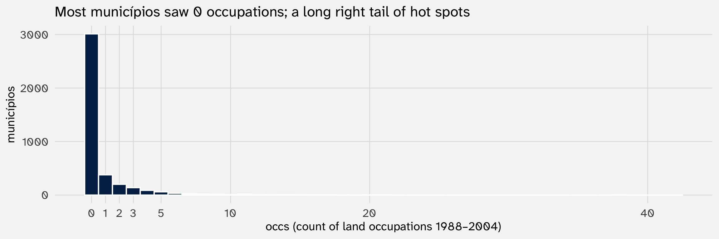
Key features:
- Non-negative integers (0, 1, 2, …)
- Mass at zero (most municípios saw no occupations)
- Long right tail (a few municípios had 20+ occupations)
- Variance grows with the mean (we’ll see this matters in §5)
Could we just use OLS?
| OLS on occs | |
|---|---|
| + p < 0.1, * p < 0.05, ** p < 0.01, *** p < 0.001 | |
| Intercept | -7.904*** |
| (0.541) | |
| landgini | 0.037*** |
| (0.004) | |
| ext_pov | -0.003 |
| (0.002) | |
| logpop | 0.616*** |
| (0.059) | |
| logarea | 0.079+ |
| (0.042) | |
| Num.Obs. | 4062 |
| R2 | 0.069 |
What OLS is doing here
When you regress a count \(Y\) on \(X\) with OLS, you are estimating the conditional mean function:
\[\mathbb{E}[Y \mid X] \;=\; X\beta\]
Read: “The expected (or average) value of Y, given X”
The estimand is well-defined:
“A one-unit increase in \(X\) changes the expected count \(\mathbb{E}[Y]\) by \(\beta\).”
That’s a meaningful, often policy-relevant quantity. Counting deaths or protests on average is exactly what a policymaker often cares about.
So: same Angrist-Pischke defense we saw with the LPM in Week 3. OLS identifies the ATE on the count scale (if your design identifies anything at all 😭)
Inequality increases the expected count of occupations
| OLS on occs | |
|---|---|
| + p < 0.1, * p < 0.05, ** p < 0.01, *** p < 0.001 | |
| Intercept | -7.904*** |
| (0.541) | |
| landgini | 0.037*** |
| (0.004) | |
| ext_pov | -0.003 |
| (0.002) | |
| logpop | 0.616*** |
| (0.059) | |
| logarea | 0.079+ |
| (0.042) | |
| Num.Obs. | 4062 |
| R2 | 0.069 |
Comparing municipalities with the same poverty rate, population, and area, municipalities with a 10 point increase in inequality (Gini) experienced (\(0.037 \times 10 = .37\)) more land occupations, on average
How big is this effect? (1/2)
All effect estimates benefit from context, but this is especially true of counts. Anchor the OLS effect against the outcome’s distribution and against a realistic shift in \(X\)
Reference numbers: \(\bar Y = 0.99\), \(\text{SD}(Y) = 3.06\). OLS slope on landgini = 0.0366.
Anchor 1 — relative to the mean of \(Y\). A 10-pp shift in landgini \(\Rightarrow\) 0.366 additional occupations.
\[\frac{10 \cdot \hat\beta_{\text{landgini}}}{\bar Y} \;=\; \frac{0.366}{0.99} \;\approx\; 36.9\%\]
→ A 10-pp Gini shift moves the expected count by ~37% of the mean município’s count.
How big is this effect? (2/2)
Anchor 2 — relative to the SD of \(Y\).
\[\frac{10 \cdot \hat\beta_{\text{landgini}}}{\text{SD}(Y)} \;=\; \frac{0.366}{3.06} \;\approx\; 0.12\;\;\text{SDs}\]
→ A 10-pp Gini shift moves the expected count by a small fraction of the outcome’s spread — a modest standardized effect.
Anchor 3 — a realistic shift in \(X\). The 25th-to-75th-percentile gap in landgini (Gini ≈ 68 to 84, a 15-pp shift):
\[\text{shift} \cdot \hat\beta_{\text{landgini}} \;=\; 15.4 \;\cdot\; 0.0366 \;\approx\; 0.565 \text{ additional occupations}\]
→ Moving a município from a typical low-inequality place to a typical high-inequality place changes expected occupations by ~0.56 — about 57% of the mean.
Whatever you do; do something!
Don’t just tell us .003 more \(Y\) when \(X\) increases by 1; draw on your data
So what’s the catch?
If OLS works for the ATE, why bother with anything else?
The same critique we leveled at the LPM in Week 3 applies here, almost line-for-line
2. Why not OLS on counts?
Four problems, parallel to W3’s “Why not the LPM?”
What’s wrong with OLS for counts?
1. Predictions can fall below zero
OLS is a line — it must eventually cross 0 for some values of \(X\). But you can’t have a negative number of occupations
2. Constant marginal effect is implausible
OLS forces \(\partial \mathbb{E}[Y] / \partial X\) to be the same when \(\mathbb{E}[Y] = 0.2\) as when \(\mathbb{E}[Y] = 200\). But effects on counts often scale with the level — changing a country from 5 protests to 6 is different from changing it from 500 to 501
3. No model of the DGP
OLS draws a line through a cloud of integer points without any claim about how counts are generated. The statistician wants a story for non-negative integer outcomes
4. Variance scales with the mean
For counts, \(\text{Var}(Y \mid X)\) typically grows with \(\mathbb{E}[Y \mid X]\) → built-in heteroskedasticity. Robust SEs help, but (the statistician would say) the deeper issue is that OLS doesn’t expect this
OLS predictions can escape below 0
augment(mod_ols) |>
  ggplot(aes(x = .fitted)) +
  geom_histogram(bins = 80, fill = "#022851", color = "white") +
  geom_vline(xintercept = 0, linetype = 2, color = "#B8611A", linewidth = 1) +
  labs(x = "OLS-predicted EXPECTED occupations per município",
       y = "municípios",
       title = "A non-trivial chunk of OLS predictions sit *below zero*")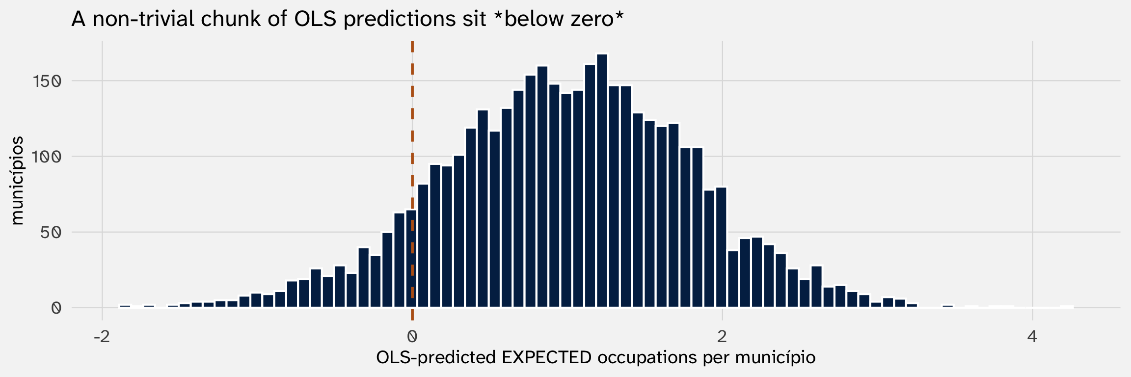
# A tibble: 1 × 1
  `municípios with predicted occs < 0`
                                 <int>
1                                  427
A line must eventually cross 0 → if predictors push downward, fitted counts go negative
Constant slopes don’t respect the floor
The OLS coefficient is the marginal effect: one number, same for everyone
So a 10-pp increase in landgini (e.g., from 65 to 75 on the rescaled Gini) always changes the expected count of occupations by the same amount, regardless of where the baseline sits:
| Baseline E[Y] | OLS effect of +10 pp landgini | New E[Y] |
|---|---|---|
| 0.1 | 0.366 | 0.466 |
| 1.0 | 0.366 | 1.366 |
| 5.0 | 0.366 | 5.366 |
| 20.0 | 0.366 | 20.366 |
The OLS shift is the same number at every baseline. Whether the baseline is 0.1 occupations (most municípios) or 20 (the hot spots), landgini adds (or subtracts) the same fixed amount
Intuitively, a constant additive effect is implausible for counts. A unit of landgini should mean something different in a high-occupation municipality than in a “quiet” one
3. The Poisson model
A model built for non-negative integer counts
The Poisson distribution
If \(Y\) is a count whose occurrences are independent and arrive at a constant rate \(\lambda\), then \(Y\) follows a Poisson distribution:
\[\Pr(Y = k) \;=\; \frac{\lambda^k \, e^{-\lambda}}{k!}, \qquad k = 0, 1, 2, \ldots\]
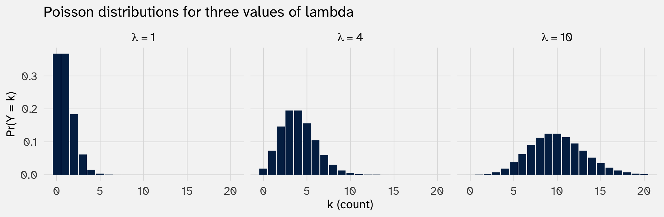
The signature property: \(\mathbb{E}[Y] = \text{Var}(Y) = \lambda\). The mean and variance are the same number
rpois() in R
rpois(n, lambda) takes \(n\) draws from a Poisson distribution with parameter \(\lambda\)
Modeling \(\lambda\) as a function of \(X\)
We want \(\lambda\) to depend on covariates. But \(\lambda > 0\) always, so we can’t write \(\lambda = X\beta\) directly — \(X\beta\) can be negative; rates can’t.
This is the same constraint problem we had with logit: the linear index \(X\beta\) is unbounded, but the parameter we want to model is bounded
Same solution: pass \(X\beta\) through a function that respects the constraint
\[\log(\lambda_i) \;=\; X_i \beta \qquad \Longleftrightarrow \qquad \lambda_i \;=\; e^{X_i \beta}\]
The exponential takes any real number and squashes it into \((0, \infty)\) → matches the constraint that \(\lambda > 0\). This is the log link
Same architecture as logit
- Logit: link is \(\log\!\frac{p}{1-p}\) (logit), inverse is \(\sigma(\cdot)\) (sigmoid). Bounds \(p \in (0,1)\).
- Poisson: link is \(\log(\lambda)\), inverse is \(\exp(\cdot)\). Bounds \(\lambda > 0\).
The link function in each case is the transformation that makes \(X\beta\) a sensible quantity.
Poisson regression in R
Same glm() call, different family:
| OLS | Poisson | |
|---|---|---|
| + p < 0.1, * p < 0.05, ** p < 0.01, *** p < 0.001 | ||
| Intercept | -7.904*** | -10.208*** |
| (0.541) | (0.213) | |
| landgini | 0.037*** | 0.054*** |
| (0.004) | (0.002) | |
| ext_pov | -0.003 | 0.002** |
| (0.002) | (0.001) | |
| logpop | 0.616*** | 0.549*** |
| (0.059) | (0.018) | |
| logarea | 0.079+ | 0.095*** |
| (0.042) | (0.012) | |
| Num.Obs. | 4062 | 4062 |
Coefficients are in log-rate units → not directly interpretable as changes in occupations
The log-rate parameterization
\[\underbrace{\log(\lambda_i)}_{\text{log expected count}} \;=\; \beta_0 + \beta_1 X_1 + \beta_2 X_2 + \cdots\]
Each \(\beta\) is the change in log expected count for a one-unit change in \(X\)
That’s not on a scale anyone thinks in. We need to convert. Three ways → next slides
Way 1: exponentiate to get a rate ratio
Take the coefficient on landgini and exponentiate it:
Interpretation: a 1-pp increase in landgini multiplies the expected count of occupations by about 1.055
For a more substantive shift — 10 pp more inequality (e.g., from Gini = 65 to 75) — multiply expected counts by:
→ roughly 1.71× the expected count
This is the rate ratio — analog to the odds ratio in logit. It’s correct, but I find rate ratios hollow without a baseline count to compare against
Way 2: predict expected counts by hand for a scenario (1/2)
To make the rate ratio concrete, fix a scenario and compute predicted counts directly
The fitted regression equation:
\[\widehat{\log \lambda_i} \;=\; -10.208 + 0.054 \cdot \text{landgini}_i + 0.002 \cdot \text{ext\_pov}_i + 0.549 \cdot \text{logpop}_i + 0.095 \cdot \text{logarea}_i\]
Scenario: an “average” município comparing low inequality (landgini = 55) to high inequality (landgini = 85)
Sample-mean controls: \(\overline{\text{ext\_pov}} = 33.5\), \(\overline{\text{logpop}} = 9.4\), \(\overline{\text{logarea}} = 6.3\).
Way 2: predict expected counts by hand for a scenario (2/2)
Low-inequality município (landgini = 55):
\[\widehat{\log\lambda} \;=\; -10.2081 + 0.0535(55) + 0.0022(33.5) + 0.5487(9.4) + 0.0948(6.3)\]
\[= -1.437 \quad\Longrightarrow\quad \hat\lambda \;=\; e^{-1.437} \;\approx\; 0.24\]
High-inequality município (landgini = 85):
\[\widehat{\log\lambda} \;=\; -1.437 + 0.0535(30) \;=\; 0.168 \quad\Longrightarrow\quad \hat\lambda \;=\; e^{0.168} \;\approx\; 1.18\]
So at sample-mean controls, the model predicts 0.24 occupations in a low-inequality município vs. 1.18 occupations in a high-inequality one
Same thing in R
Vary landgini, hold others fixed
scenario = crossing(
  landgini = seq(0, 100, by = 5),
  logpop   = mean(inv_clean$logpop),
  ext_pov  = mean(inv_clean$ext_pov),
  logarea  = mean(inv_clean$logarea)
)

preds = predictions(mod_pois, newdata = scenario, type = "response")

preds |>
  as_tibble() |>
  select(estimate, conf.low, conf.high, landgini, logpop, ext_pov, logarea)
# A tibble: 21 × 7
estimate conf.low conf.high landgini logpop ext_pov logarea
<dbl> <dbl> <dbl> <dbl> <dbl> <dbl> <dbl>
1 0.0122 0.00888 0.0156 0 9.35 33.5 6.30
2 0.0160 0.0119 0.0201 5 9.35 33.5 6.30
3 0.0209 0.0159 0.0259 10 9.35 33.5 6.30
4 0.0273 0.0212 0.0334 15 9.35 33.5 6.30
5 0.0357 0.0283 0.0431 20 9.35 33.5 6.30
6 0.0466 0.0377 0.0556 25 9.35 33.5 6.30
7 0.0610 0.0503 0.0717 30 9.35 33.5 6.30
8 0.0797 0.0670 0.0923 35 9.35 33.5 6.30
9 0.104 0.0893 0.119 40 9.35 33.5 6.30
10 0.136 0.119 0.153 45 9.35 33.5 6.30
# ℹ 11 more rowsThe estimate column is \(\hat\lambda\) → the expected count of land occupations for that scenario, with a 95% CI
Remember rounding
The by-hand examples in class won’t match R output exactly because of rounding, but the math/logic is the same
Visualize it
The same scenario plotted across the full range of landgini:
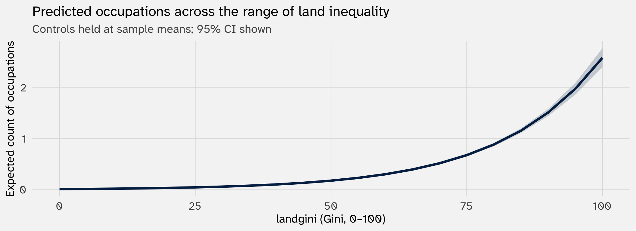
The curve bends upward as landgini grows — predicted counts rise faster at higher inequality.
That convex shape is what the log link delivers: a constant percentage effect of \(X\) produces ever-larger absolute effects as \(\lambda\) grows
Way 3: the marginal effect, via calculus
Same calculus move from Week 3, applied to the new model
We want \(\partial \lambda / \partial X\). Start from the link:
\[\lambda \;=\; e^{X\beta}\]
Differentiate using the chain rule (derivative of \(e^u\) is \(e^u \cdot u'\)):
\[\frac{\partial \lambda}{\partial X} \;=\; e^{X\beta} \cdot \beta \;=\; \lambda \cdot \beta\]
\[\boxed{\;\;\frac{\partial \lambda}{\partial X} \;=\; \beta \cdot \lambda\;\;}\]
The marginal effect of \(X\) on the expected count scales with \(\lambda\) itself. Not constant.
What this looks like
The same shape we saw in Week 2 with \(\log(Y) = \beta_0 + \beta_1 X\):
The effect of \(X\) is proportional to the level of \(Y\). Big \(\lambda\) → big absolute effect; small \(\lambda\) → small absolute effect.
The log link delivers a multiplicative response: counts respond to \(X\) multiplicatively, not additively
Concretely:
- A quiet município with \(\lambda = 1\) occupation → a unit of \(X\) adds about 0.05 occupations
- A hot spot with \(\lambda = 100\) occupations → a unit of \(X\) adds about 5 occupations
So the effect grows with the rate → inequality should increase occupations more easily in a place with a higher expected count (given covariates)
By hand: same \(\hat\beta\), three different MEs across scenarios
For our fitted model, hold the controls at sample means; vary landgini:
b   = coef(mod_pois)
mns = c(mean(inv_clean$ext_pov), mean(inv_clean$logpop), mean(inv_clean$logarea))

tibble(landgini = c(55, 75, 95)) |>
  mutate(
    eta          = b["(Intercept)"] + b["landgini"] * landgini +
                   b["ext_pov"] * mns[1] + b["logpop"] * mns[2] + b["logarea"] * mns[3],
    lambda       = exp(eta),
    beta_landgini= b["landgini"],
    ME_landgini  = beta_landgini * lambda
  )
# A tibble: 3 × 5
landgini eta lambda beta_landgini ME_landgini
<dbl> <dbl> <dbl> <dbl> <dbl>
1 55 -1.46 0.232 0.0535 0.0124
2 75 -0.388 0.678 0.0535 0.0363
3 95 0.683 1.98 0.0535 0.106 Same \(\hat\beta_{\text{landgini}}\). Three different MEs, because \(\lambda\) changes across scenarios. The bigger the baseline expected count, the bigger the absolute effect of 1 pp more landgini on that count
Visualize: ME of landgini across the data
slopes() computes \(\partial\lambda/\partial X\) at every scenario and plots how the ME varies:
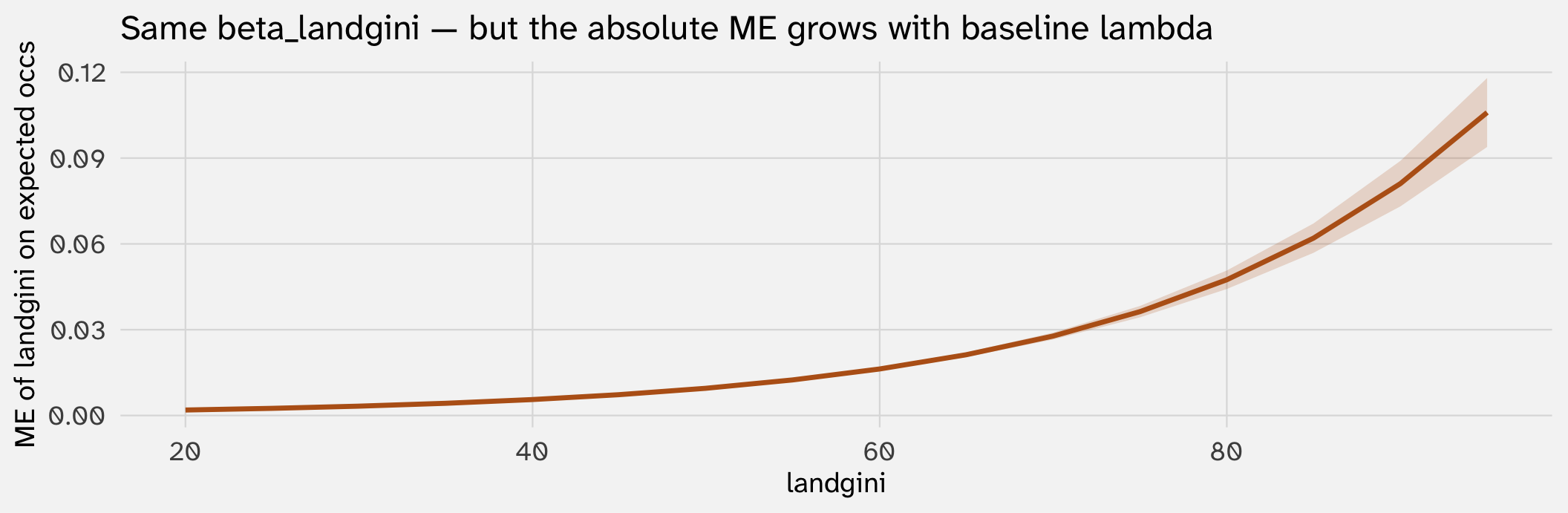
This is the same picture as the logit ME plot from Week 3. Same calculus: one \(\hat\beta\), many MEs across the predictor’s range
What if I think effects are diminishing, not multiplicative?
Plain Poisson commits to one shape: effects scale with \(\lambda\) (multiplicative growth). What if your theory predicts the opposite — diminishing returns with effects flattening as \(\lambda\) grows?
Same situation as Week 4 logit interactions
In an additive logit, the effect of X depended on Z only through the scaling factor \(p(1-p)\) — a constrained, symmetric moderation. To get richer moderation, you added an explicit \(X \cdot Z\) product term
Same move here. Plain Poisson commits to multiplicative growth. To get a different shape, add it explicitly:
- Quadratic in X: \(\exp(\beta_1 X + \beta_2 X^2)\) → marginal effect can flatten and reverse sign (inverted-U story)
- log(X) as predictor: \(\exp(\beta_0 + \beta_1 \log X)\) → marginal effect \(\beta_1 \lambda / X\) strictly shrinks with X (pure diminishing returns, no reversal)
- Interactions \(X \cdot Z\) → effect varies by group / baseline level
The general lesson: every model imposes a structural shape. If your theory says something different, add the structure explicitly
The AME — one number for the paper
Average across the empirical distribution of the data:
 Estimate Std. Error    z Pr(>|z|)     S  2.5 % 97.5 %
   0.0531    0.00188 28.2   <0.001 577.4 0.0494 0.0568

Term: landgini
Type: response
Comparison: dY/dX
The average ME of landgini on expected occupations, averaged across all 4,062 municípios. This is the headline quantity
→ On average across municípios, a 1-pp increase in landgini is associated with about 0.0531 additional expected land occupations, holding poverty, population, and area fixed.
Apply the same anchoring as before (mean, SD, percentile shift) to translate this AME into a substantive story; the framework from §1 transfers directly
The Poisson workflow: fit, convert, report
- Fit:
glm(Y ~ X + controls, family = poisson) - Don’t report raw coefficients as effects (they’re log-rates); appendix
- Plot predicted counts across your key predictor, holding controls at sensible values
- Report the AME (or AMC for categorical) as your top-level number
- Check the variance assumption (next: §5)
Common pitfalls with Poisson
1. Don’t read \(\beta\) as a count change. It’s in log-rate units. Always convert (rate ratio, scenario, AME)
2. There is no single “effect.” The marginal effect depends on baseline \(\lambda\) → same as logit’s “depends on baseline \(p\)”
3. Predicted counts can be very small for some scenarios. The “rate” \(\lambda\) is the expected count, not the most likely count. For rare events, \(\hat\lambda < 1\) is common — it means a \(\hat\lambda\) fraction of an event on average
When does Poisson = OLS?
Same setup as the LPM=logit comparison from Week 3. Make a binary indicator from landgini (above vs. below median) and fit both models with no other controls:
| high_gini | OLS | Poisson |
|---|---|---|
| 0 | 0.501 | 0.501 |
| 1 | 1.483 | 1.483 |
Identical → with one binary predictor and no controls, both models just compute group means
When does Poisson not equal OLS?
Add the controls back in:
| high_gini | OLS | Poisson | diff |
|---|---|---|---|
| 0.0 | 0.547 | 0.444 | -0.104 |
| 0.5 | 0.992 | 0.728 | -0.264 |
| 1.0 | 1.436 | 1.194 | -0.242 |
Close, not identical → divergence grows where the log link bends and the OLS straight line cannot
→ Poisson = OLS when: the model is saturated. Once you add real controls, the link function starts doing work and the predictions diverge
What does “saturated” mean?
A regression model is saturated when it has as many parameters as there are unique combinations of predictor values. With one binary X plus an intercept, you have 2 parameters and exactly 2 covariate cells (X = 0 and X = 1). A saturated model can hit each cell mean exactly, so any link function produces the same predictions — there’s nothing left for the link to interpolate over. Add a continuous control (or a second covariate), and the model becomes non-saturated; the link function starts doing real work.
Back to the debate between “economists” and “statisticians”
The “saturated → models agree” insight maps onto the methodological divide we flagged in Week 3
The economist
Wants design-based inference — an experiment (real or natural), an IV, a DiD, an RDD
If the design identifies the effect, not much hangs on controls → models stay close to saturated
The ideal estimator is just a difference in means. The link function doesn’t matter much because you’re already close to the saturated case → OLS gives the ATE on the count scale and that’s what you wanted
→ defaults to OLS even with binary or count \(Y\)
The statistician
Wants to model the DGP — match the model’s structure to how \(Y\) is actually generated (Bernoulli for binaries, Poisson/NB for counts, …)
A lot hangs on the variables in the model: each variable adds parameters but also forces a functional shape via the link → models are non-saturated and link functions do real work
→ defaults to GLM (logit / Poisson / NB) matched to the outcome type
Aggressive oversimplification (still!)
Lots of economists model DGPs; lots of statisticians do design-based work. This is a methodological caricature, useful for sharpening the trade-offs
4. MLE for Poisson — application
The same Week 4 machinery, with a new likelihood plugged in
Same framework, new likelihood
Week 4: MLE means maximize the likelihood. To apply it to Poisson, we just need to write down the right likelihood
For one observation: the Poisson PMF gives the probability of seeing \(Y_i\) deaths/occupations/protests/etc. given \(\lambda_i\):
\[\Pr(Y_i \mid X_i, \beta) \;=\; \frac{\lambda_i^{Y_i} \, e^{-\lambda_i}}{Y_i!}, \qquad \lambda_i = e^{X_i'\beta}\]
For all \(n\) independent observations, the joint likelihood is the product:
\[\mathcal{L}(\beta) \;=\; \prod_{i=1}^n \frac{\lambda_i^{Y_i} \, e^{-\lambda_i}}{Y_i!}\]
Take logs, drop constants
Same trick as logit: take the log to convert products into sums
\[\ell(\beta) \;=\; \log \mathcal{L}(\beta) \;=\; \sum_{i=1}^n \Bigl[ Y_i \log \lambda_i \;-\; \lambda_i \;-\; \log(Y_i!) \Bigr]\]
The \(\log(Y_i!)\) term doesn’t depend on \(\beta\) → drop it. Substitute \(\lambda_i = e^{X_i'\beta}\):
\[\ell(\beta) \;=\; \sum_{i=1}^n \Bigl[ Y_i \cdot X_i'\beta \;-\; e^{X_i'\beta} \Bigr]\]
This is the function glm() is climbing when you ask for a Poisson model. The architecture is the same as logit; only the function changed.
Try different \(\beta\) vectors
The log-likelihood is just a function of \(\beta\): plug in a vector, get a number. Try a few:
b_mle = coef(mod_pois)  # the MLE from glm()

# Poisson log-likelihood (modulo the constant that drops out)
loglik_pois = function(b) {
  eta = b[1] + b[2]*inv_clean$landgini + b[3]*inv_clean$ext_pov +
        b[4]*inv_clean$logpop + b[5]*inv_clean$logarea
  sum(inv_clean$occs * eta - exp(eta))
}

tibble(
  candidate = c("All zeros",
                "Intercept only at log(mean Y)",
                "MLE (the peak)",
                "Flipped signs"),
  log_lik   = c(loglik_pois(c(0, 0, 0, 0, 0)),
                loglik_pois(c(log(mean(inv_clean$occs)), 0, 0, 0, 0)),
                loglik_pois(b_mle),
                loglik_pois(-b_mle)) |> round(0)
)
# A tibble: 4 × 2
candidate log_lik
<chr> <dbl>
1 All zeros -4062
2 Intercept only at log(mean Y) -4062
3 MLE (the peak) -2638
4 Flipped signs -11567What you get back
Same outputs as Week 4:
- \(\hat\beta\) from Newton–Raphson on \(\ell(\beta)\)
- SEs from \(\sqrt{\text{diag}(\mathcal{I}^{-1})}\) where \(\mathcal{I} = -\ell''(\hat\beta)\)
- A note:
Number of Fisher Scoring iterations: k
Call:
glm(formula = occs ~ landgini + ext_pov + logpop + logarea, family = poisson,
    data = inv_clean)

Coefficients:
              Estimate Std. Error z value Pr(>|z|)
(Intercept) -1.021e+01  2.134e-01 -47.840  < 2e-16 ***
landgini     5.354e-02  1.703e-03  31.430  < 2e-16 ***
ext_pov      2.229e-03  8.416e-04   2.648  0.00809 **
logpop       5.487e-01  1.764e-02  31.114  < 2e-16 ***
logarea      9.478e-02  1.205e-02   7.866 3.67e-15 ***
---
Signif. codes:  0 '***' 0.001 '**' 0.01 '*' 0.05 '.' 0.1 ' ' 1

(Dispersion parameter for poisson family taken to be 1)

    Null deviance: 15008  on 4061  degrees of freedom
Residual deviance: 12160  on 4057  degrees of freedom
AIC: 15128

Number of Fisher Scoring iterations: 6Review: so far
What are we trying to do?
\[\eta_i = \beta_0 + \beta_1 \cdot X1_i + \beta_2 \cdot X2_i + \dots\]
We are trying to estimate a model that is linear in the parameters → data and coefficients enter the model additively, even if the model (logit, Poisson) or our specification (interactions, quadratic) are non-linear
The problem
Binary outcome (logit)
\(Y \in \{0, 1\}\)
We need \(\eta\) to map onto a probability → must live in \([0, 1]\)
Why? We believe the DGP is Bernoulli — given a probability \(p\), nature flips a coin
So whatever \(\eta\) produces has to land in \([0, 1]\) — that’s the parameter the DGP takes
Count outcome (Poisson)
\(Y \in \{0, 1, 2, 3, \ldots\}\)
We need \(\eta\) to map onto a rate → must be \(> 0\)
Why? We believe the DGP is Poisson — given a rate \(\lambda\), nature draws a count
So whatever \(\eta\) produces has to be \(> 0\) — that’s the parameter the DGP takes
But \(\eta = X\beta\) can take any real value, \((-\infty, +\infty)\) → it doesn’t naturally live where the DGP’s parameter needs to live
The solution: pass \(\eta\) through a function
Logit: the sigmoid
\[p = \sigma(\eta) = \frac{1}{1 + e^{-\eta}}\]
Squashes \((-\infty, +\infty) \to (0, 1)\)
Poisson: exponentiate
\[\lambda = e^{\eta}\]
Maps \((-\infty, +\infty) \to (0, +\infty)\)
In both cases, the linear predictor stays linear → we just transform it at the end so the output lands in the right space
How do we pick \(\beta\)? Maximum likelihood
Pick the \(\beta\) that makes the observed data most likely under the model
Logit log-likelihood
\[\eta_i = X_i\beta, \quad p_i = \sigma(\eta_i)\]
\[\ell(\beta) = \sum_i \bigl[\, y_i \log p_i + (1 - y_i)\log(1 - p_i) \,\bigr]\]
Poisson log-likelihood
\[\eta_i = X_i\beta, \quad \lambda_i = e^{\eta_i}\]
\[\ell(\beta) = \sum_i \bigl[\, y_i \, \times \eta_i - e^{\eta_i} \,\bigr] \]
Toy data; two candidate \(\beta\) vectors. Which one fits better?
\(X = (0, 1, 2), \quad Y = (0, 1, 1)\)
| candidate \((\beta_0, \beta_1)\) | \(\ell(\beta)\) |
|---|---|
| \((-1, \;1)\) | \(-1.32\) |
| \(\mathbf{(-2, \;2)}\) | \(\mathbf{-0.95}\) ← higher |
\(X = (0, 1, 2), \quad Y = (1, 2, 4)\)
| candidate \((\beta_0, \beta_1)\) | \(\ell(\beta)\) |
|---|---|
| \((0, \;0.5)\) | \(-0.37\) |
| \(\mathbf{(0, \;0.7)}\) | \(\mathbf{-0.07}\) ← higher |
The MLE is the \(\beta\) that maximizes \(\ell\) — glm() uses the same Newton-Raphson search from Week 4 to find it
So what scale are the coefficients on?
Logit → log-odds
\[\log\!\left(\frac{p}{1 - p}\right) = \beta_0 + \beta_1 X_1 + \dots\]
A 1-unit change in \(X_1\) shifts the log-odds of \(Y = 1\) by \(\beta_1\)
Poisson → log-rates
\[\log(\lambda) = \beta_0 + \beta_1 X_1 + \dots\]
A 1-unit change in \(X_1\) shifts the log-rate of \(Y\) by \(\beta_1\)
This is why raw coefficients are not directly interpretable — they sit on the link scale, not the outcome scale
Getting back to something sensible
Suppose for both models: \(\hat\beta_0 = -1\), \(\hat\beta_1 = 0.5\), and we ask about \(X_1 = 4\)
Step 1 — compute \(\eta\) (same for both):
\(\eta = -1 + 0.5 \cdot 4 = 1\)
Logit: η → probability
Step 2 — sigmoid:
\[\hat p = \frac{1}{1 + e^{-\eta}} = \frac{1}{1 + e^{-1}}\]
\[\hat p = \frac{1}{1 + 0.37} \approx \mathbf{0.73}\]
→ predicted probability of \(Y = 1\) is about 73%
Poisson: η → rate
Step 2 — exponentiate:
\[\hat\lambda = e^{\eta} = e^{1}\]
\[\hat\lambda \approx \mathbf{2.72}\]
→ predicted count of \(Y\) is about 2.72 events
Same \(\eta\), two different outcome scales → the link function is what does the translation
5. Adjustments to Poisson: overdispersion
When the mean does not equal the variance
The Poisson assumption
The Poisson distribution has a single parameter \(\lambda\) that controls both the mean and the variance:
\[\mathbb{E}[Y] \;=\; \text{Var}(Y) \;=\; \lambda\]
For Poisson to fit, the conditional variance of \(Y\) at each \(X\) must equal the conditional mean
Does the assumption hold for our data?
There’s a metric for this: the dispersion statistic \(\hat\phi\), built from Pearson residuals
\[\hat\phi \;=\; \frac{1}{n - k} \sum_i \frac{(Y_i - \hat\lambda_i)^2}{\hat\lambda_i}\]
If Poisson holds, \(\hat\phi \approx 1\). If the data are more spread than Poisson predicts, \(\hat\phi > 1\)
The data are 7× more spread than Poisson predicts — variance massively outpaces the predicted rate
Why this matters
If \(\text{Var}(Y) > \lambda\) but the model assumes \(\text{Var}(Y) = \lambda\), the model underestimates uncertainty
Concretely: SEs are too small → \(z\)-stats too big → \(p\)-values too small → false confidence
This is similar to the LPM heteroskedasticity story
Week 3 with the LPM: binary \(Y\) has built-in \(p(1-p)\) heteroskedasticity → classical SEs too small → use HC2 robust SEs.
Week 5 with Poisson: count \(Y\) has built-in mean-variance link → if it’s misspecified, variance is too small → SEs too small.
Same diagnosis pattern: the model imposes a variance assumption that the data don’t satisfy.
Two fixes, escalating in ambition
Fix 1 — quasi-Poisson / robust SEs
Keep the Poisson coefficients, but multiply SEs by \(\sqrt{\hat\phi}\) to account for overdispersion. This is exactly what quasipoisson does:
# A tibble: 5 × 5
  term         estimate std.error statistic  p.value
  <chr>           <dbl>     <dbl>     <dbl>    <dbl>
1 (Intercept) -10.2       0.568     -18.0   1.62e-69
2 landgini      0.0535    0.00454    11.8   1.21e-31
3 ext_pov       0.00223   0.00224     0.995 3.20e- 1
4 logpop        0.549     0.0470     11.7   4.72e-31
5 logarea       0.0948    0.0321      2.95  3.15e- 3
Fix 2 — change the DGP
Use a distribution that allows variance to exceed the mean. The standard choice: Negative Binomial → §6
6. The Negative Binomial model
A count distribution where variance and mean can move independently
NB unties the variance from the mean
Poisson: \(\text{Var}(Y) = \mu\) (the mean). One number, two jobs
Negative Binomial:
\[\text{Var}(Y) \;=\; \mu \;+\; \frac{\mu^2}{\theta}\]
where \(\theta > 0\) is a separate dispersion parameter (sometimes called “size”). It controls how much extra variance there is beyond what Poisson would give
- \(\theta \to \infty\) → second term vanishes → NB collapses to Poisson
- \(\theta\) small → variance much larger than mean → strongly overdispersed
What the variance looks like
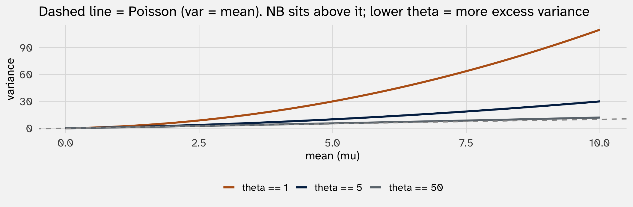
The dashed line is Poisson. NB curves climb above it; how steeply depends on \(\theta\). Smaller \(\theta\) → more overdispersion
Fit a Negative Binomial in R
| Poisson | Quasi-Poisson | Negative Binomial | |
|---|---|---|---|
| + p < 0.1, * p < 0.05, ** p < 0.01, *** p < 0.001 | |||
| Intercept | -10.208*** | -10.208*** | -10.476*** |
| (0.213) | (0.568) | (0.523) | |
| landgini | 0.054*** | 0.054*** | 0.054*** |
| (0.002) | (0.005) | (0.004) | |
| ext_pov | 0.002** | 0.002 | -0.001 |
| (0.001) | (0.002) | (0.002) | |
| logpop | 0.549*** | 0.549*** | 0.539*** |
| (0.018) | (0.047) | (0.051) | |
| logarea | 0.095*** | 0.095** | 0.159*** |
| (0.012) | (0.032) | (0.035) | |
| Num.Obs. | 4062 | 4062 | 4062 |
Coefficients are usually close across all three. What differs is the standard errors → much larger under quasi-Poisson and NB, because they both acknowledge the extra variance
Same interpretation, more realistic uncertainty
Coefficient interpretation is identical to Poisson:
- Log-rate units → exponentiate for rate ratios
- Marginal effect: \(\partial \lambda / \partial X = \beta \cdot \lambda\)
- All the Week 3-style workflow transfers (slopes, comparisons, AME, contextualization)
What changes:
- CIs are wider (correctly so; Poisson’s were artificially narrow)
- \(z\)-stats and \(p\)-values reflect more honest uncertainty
Count-model toolkit
| Outcome features | Model | R call |
|---|---|---|
| Counts, \(\text{Var} \approx \mathbb{E}[Y]\), design identifies ATE | OLS (with HC robust SEs) | lm_robust() |
| Counts, \(\text{Var} = \mathbb{E}[Y]\) holds | Poisson | glm(family = poisson) |
| Counts, \(\text{Var} > \mathbb{E}[Y]\) (the usual case) | Negative Binomial | MASS::glm.nb() |
For most political-science count outcomes, quasi-Poisson or NB is the right default